1. Pixels and Linear Filters
Image Formation Process
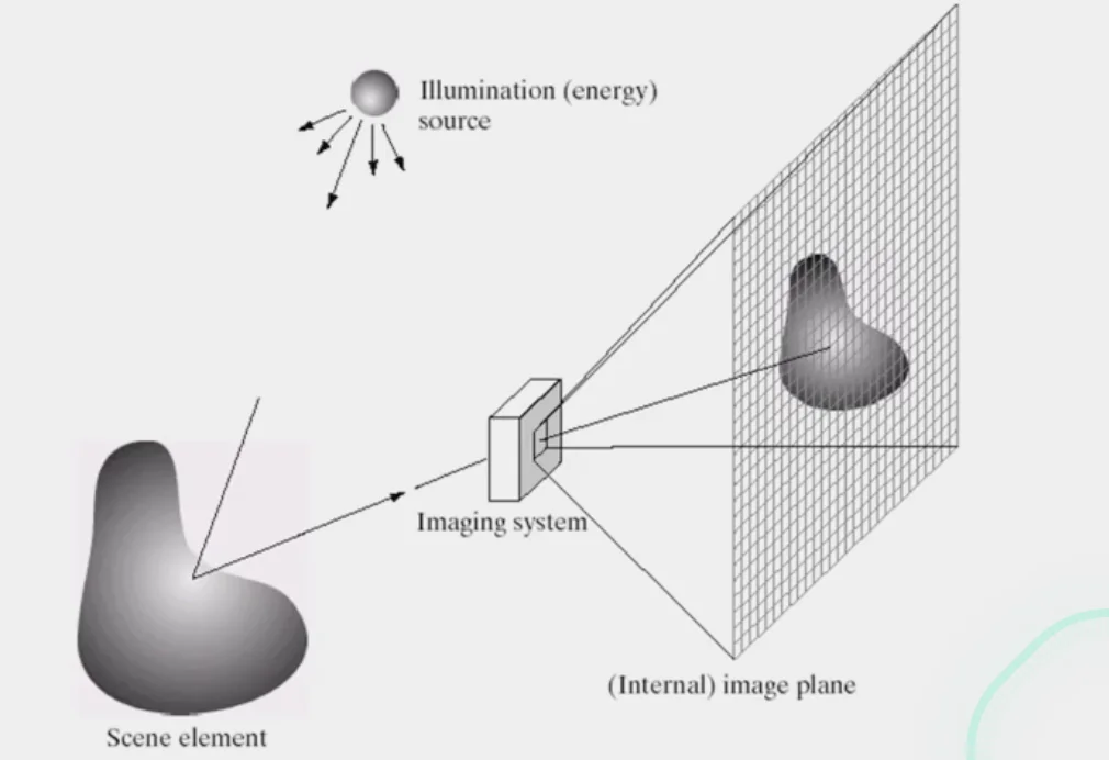
- Light comes out from the sources
- Light bounces off the elements in the scene
- Some of that light is reflected through the lens into the camera onto the imaging plane
Note
Films and Analog Camera:
- Light is recorded as a continuous signal on that film
Digital Camera
- Light is recorded onto a CCD
- Cells in CCD are photo-recepters converting the photrons of light into electrons
Sensor Array
- Continuous signals recorded are discretized based on
spaceandintensity
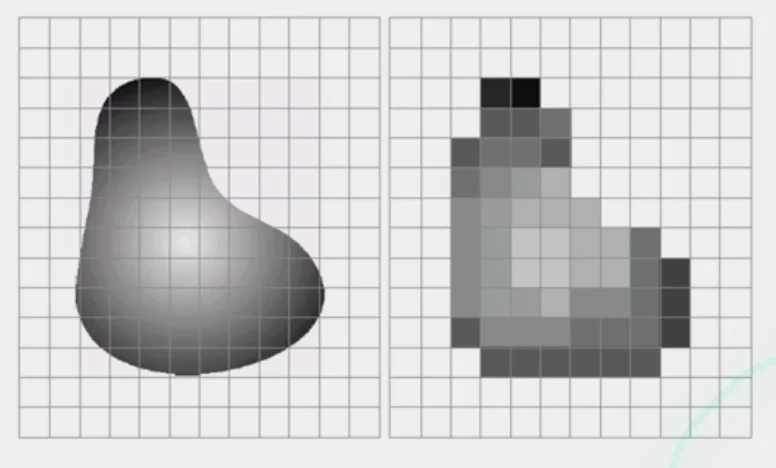
The raster image (pixel matrix)
- Raster Image: the matrix representation of an image
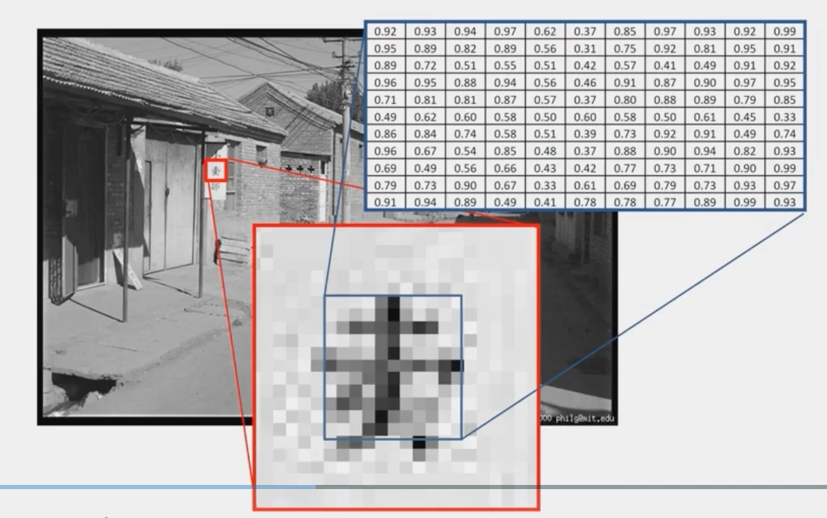
- Difficult Part for image analysis:
- We perceive the contrast of a
blackcharacter with awhitebackground - In reality, it’s a
mid-rangecharacter with anoisybackground
Perception of Intensity
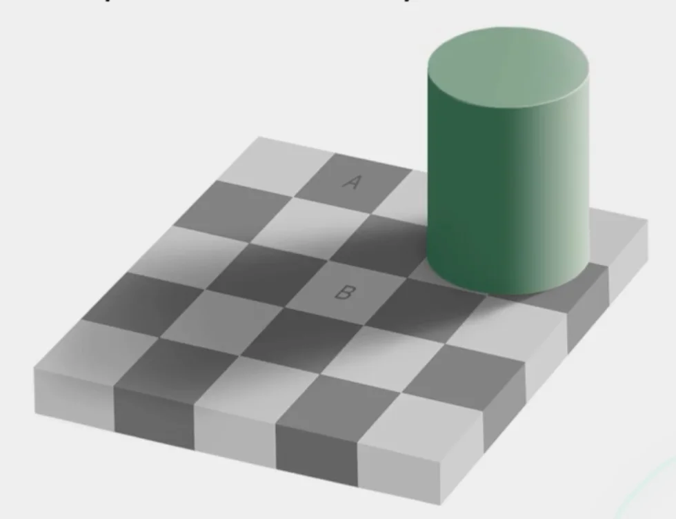
- Intensity: Overall, how much light is coming over the sensor.
- The
darknessof A and B is actually the same.
Digital Color Images
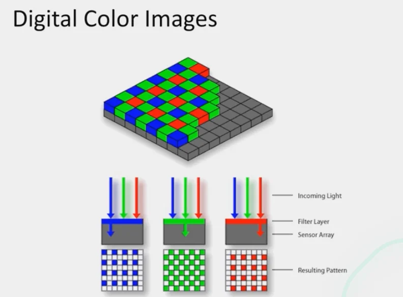
- Color images are all generated with 3 different colors with different intensity
Images in Python
# read image (order: BGR)
im = cv2.imread(filename)

# order channels as RGB
im = cv2.cvtColor(im, cv2.COLOR_BGR2RGB)
im = im / 255- RGB image
imisH x W x 3matrix (np.ndarray) H: heightW: width3: # of channels (RGB)im[0, 0, 0]:- top-left pixel value in the R-channel
im[y, x, c]:y + 1pixels downx + 1pixels rightcth channel
Image Filtering
What is it?
- compute function of local neighborhood at each position
Example: Box Filter
- Blurring image
- Calculating moving average
Formula
How it works
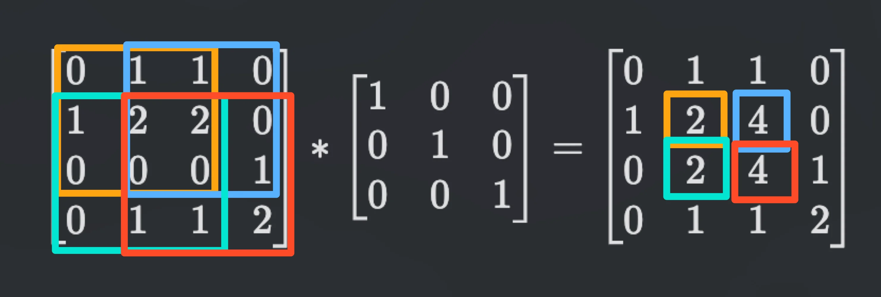
- Let’s say you have a
3 x 3box filter
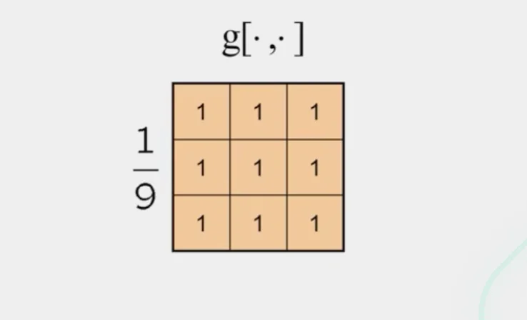
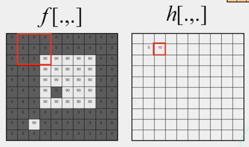
- For every
3 x 3window in the image,
- multiply the corresponding elements of that patch of the image with the elements in the filters
- sum up all of products
Types of Filters
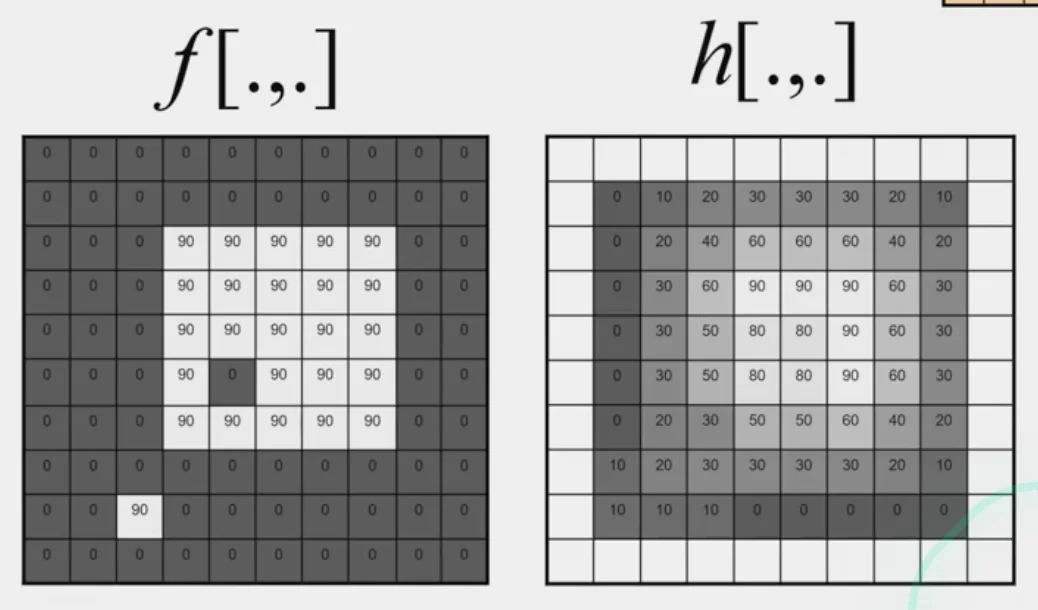
Box Filter
- smooth the image
- create some edges (will be explained later in the course)
Calculate by hand
Note: convolution
Practice with Linear Filters
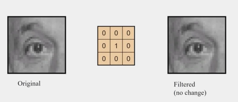
Identity Filter
- no change
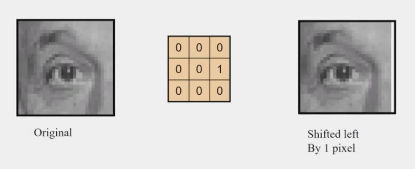
Shifted Left
- every pixel would be replaced by its right neighbor
Sharpening
- accentuates differences with local average
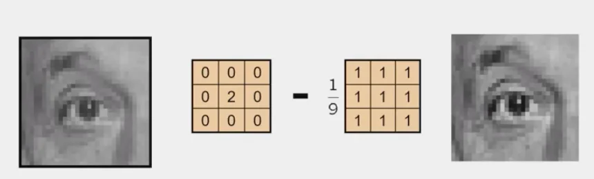
Tip
You are calculating the original matrix + the difference of the center pixel from the average of the neighbors, which makes the differences stronger.
Edge Filter
- Subtracting sum of pixels to the left to sum of the pixels to the right
- Stronger left pixels -> positive result
- Stronger right pixels -> negative result
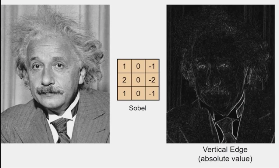
white pixels: high magnitudeblack pixels: low magnitude
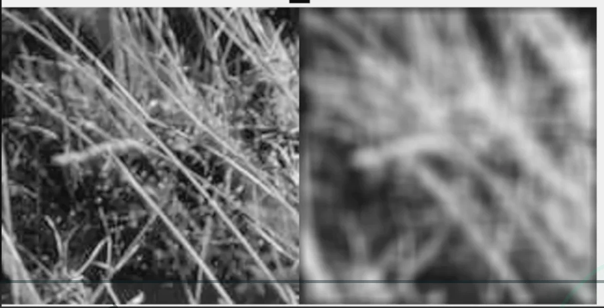
How to synthesize motion blur?
- Shift the picture by multiple positions and then average those out
im = cv2.imread(im_fn)

# invert to gray scale
im = cv2.cvtColor(im, cv2.COLOR_BGR2GRAY) / 255

# degree motion blur
theta = 45
# theta = 0 # vertical filter
# theta = 90 # horizontal filter
len = 15
mid = (len - 1) / 2

fil = np.zeros((len, len))
fil[:, int(mid)] = 1 / len # sum of the values is 1
R = cv2.getRotationMatrix2D((mid, mid), theta, 1)
fil = cv2.wrapAffine(fil, R, (len, len))

im_fil = cv2.filter2D(im, -1, fil)
fig, axes = plt.subplot(3, 1, figsize=(50, 50))
axes[0].imshow(im, cmap='gray')
axes[1].imshow(fil, cmap='gray)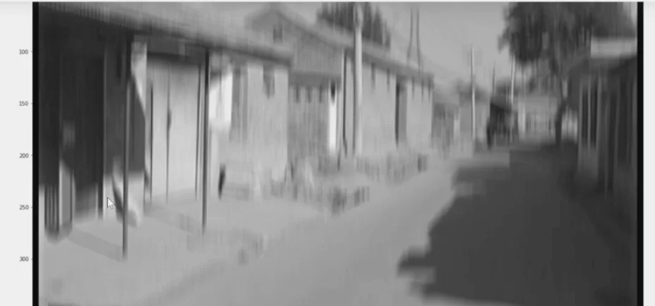
Warning
This cannot be used to anti-blur the image as there are several ways tThat may lead to the same blurred image.
If we change the len
- The amount of blur would be less
len = 7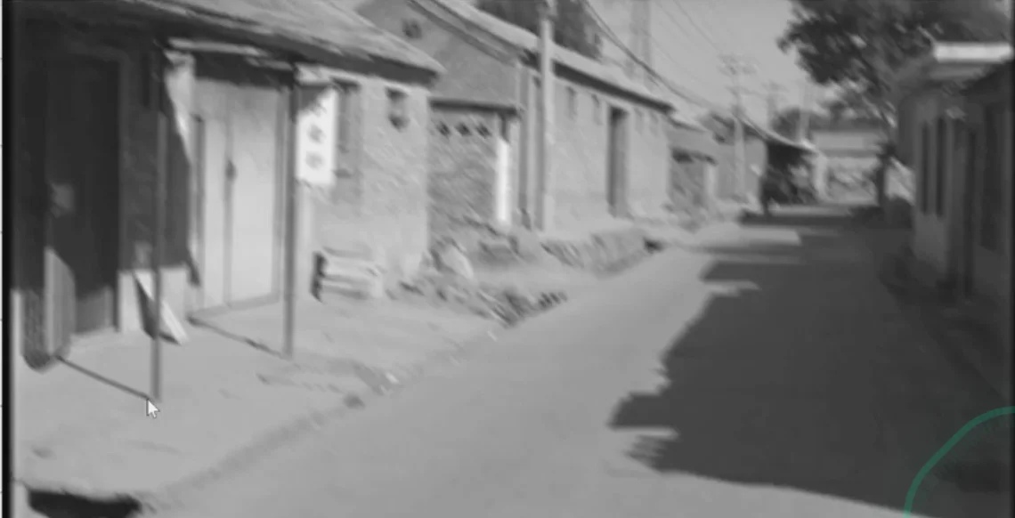
If we do not include the all rows
alpha = 45
len = 25
fil[12:, int(mid)] = 1 / len # synthesizing blur on the right half only
R = cv2.getRotationMatrix2D((mid, mid), theta, 1)
fil = cv2.wrapAffine(fil, R, (len, len))- The pixels on the upper-left will be replaced by the pixels on the lower-right
- The image would be shifted to the upper-left and blurred

Correlation vs. Convolution
2d correlation
im_fil = cv2.filter2d(im, -1, fil)- When you takes a window over the image, you multiply corresponding elements of that window with the elements of the
kernel(filter matrix) or the filter.
2d convolution
im_fil = scipy.signal.convolve2d(im, fil, [opts])- Convolution flip the kernel by 180 degrees first and then apply correlation
Important
“convolve” mirrors the kernel, while “filter” doesn’t. The following two expressions are the same
cv2.filter2D(im, -1, cv2.flip(fil, -1))siginal.convolve2d(im, fil, mode='same', boundary='symm')
Properties of Linear Filters
Linearity
Shift Invariance:
- Same behavior regardless of pixel location
Note
Any linear, shift-invariant filter’s operations can be represented as convolutions
Commutative
Associative
Distributes over addition
Scalars factor out:
Identity
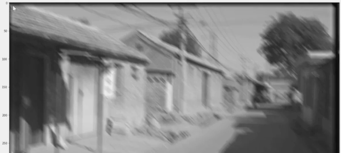
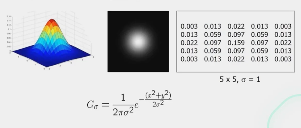
Gaussian Filter
- Weight contributions of neighboring pixels by nearness
- The value in the center is the highest
- It is a very effective smoother
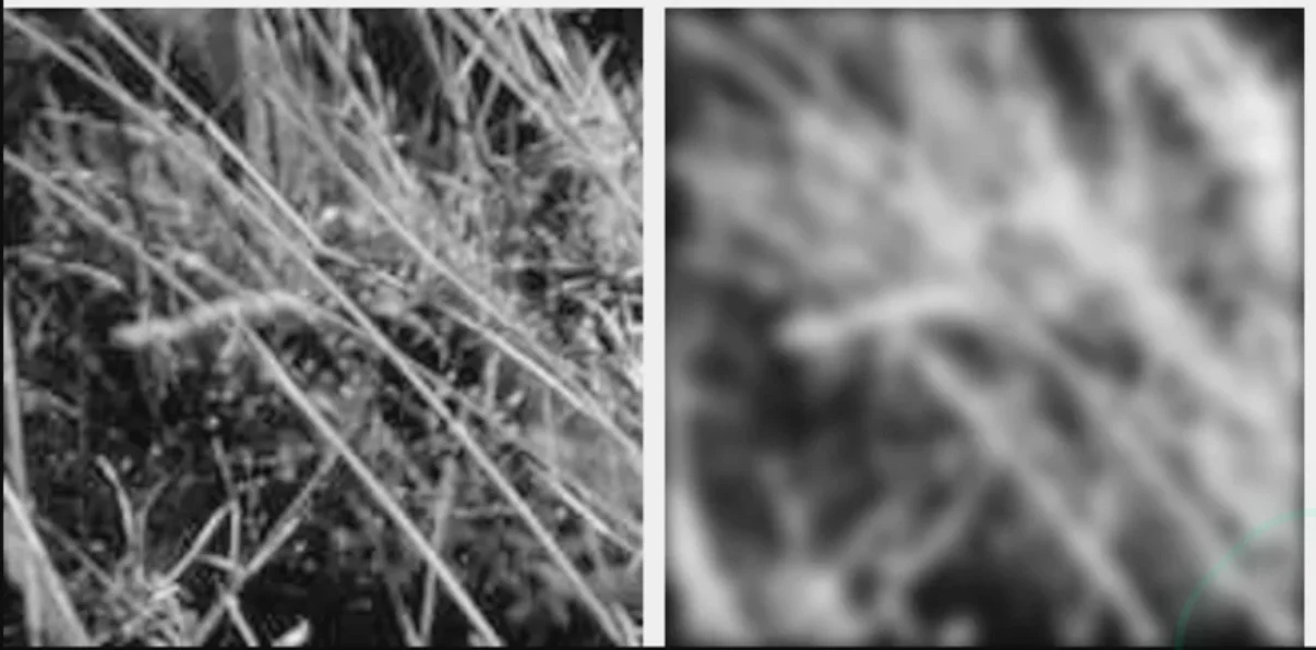
- Remove the
high-frequencycomponents from the image (low-pass filter)
Convolution with self is another Gaussian
- convolving two times with Gaussian kernel of width is the same as convolving once with kernel of width
- The Gaussian kernel is defined as:
- Convolving two Gaussian functions = Multiplying their Fourier transforms.
- The Fourier transform of a Gaussian is also a Gaussian:
Convolve two Gaussians with widths and :
- In frequency domain:
- This corresponds to a Gaussian with variance
- For two identical Gaussians with width σ:
Separability of the Gaussian Filter
Separability Example
- Faster to computer
method 1takes times of caluculationmethod 2takes times of calculation
Practical Matters
Proper size for kernel
- For kenel, with a proper size, the values at edges should be near zero
- For Gaussian:
Near the edges
- the filter window falls off the edge of the image
Extrapolation
clip filter
- apply smoothing filter
- Crop the image back to the original size
wrap around
copy edge
Caution
For templating matching, the copied edges may cause some extra problems
reflect across edge
In Python
Methods
convolve2d(g, f, boundary='fill', 0) # clip filter
convolve2d(g, f, boundary='wrap') # wrap around
convolve2d(g, f, boundary='symm') # reflect across edge
Size of output
-
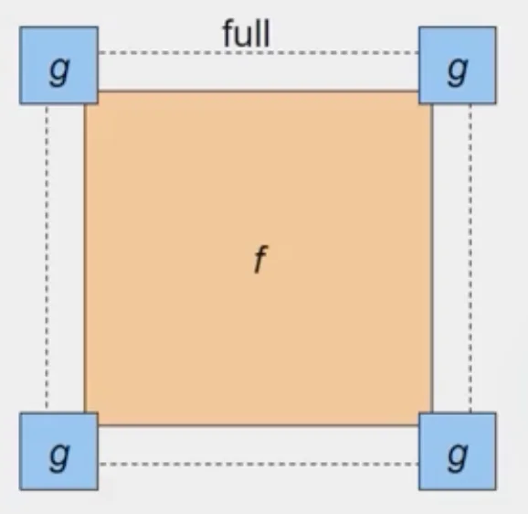
convolve2d(g, f, mode) -
mode='full': -
output size is
sumof sizes offandg
-
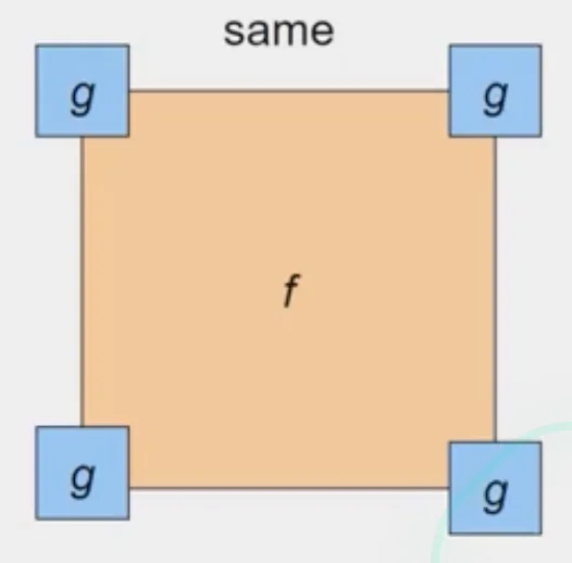
mode='same': -
output size is the same as
f -
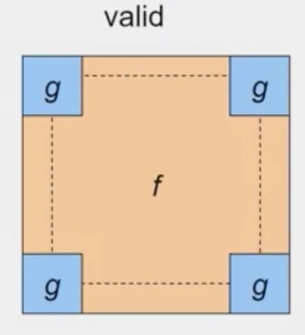
What we usually wanna do
-
mode='valid' -
output size is the
differenceof sizes offandg
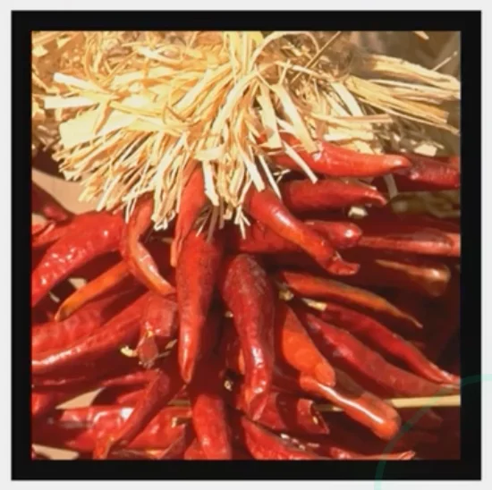
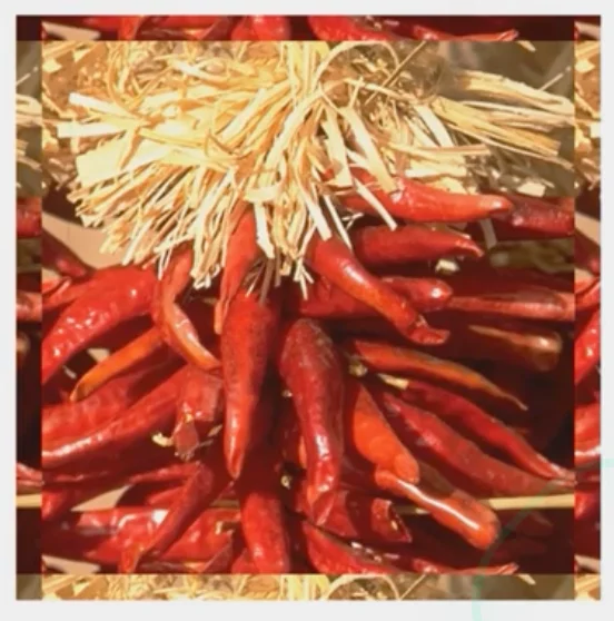
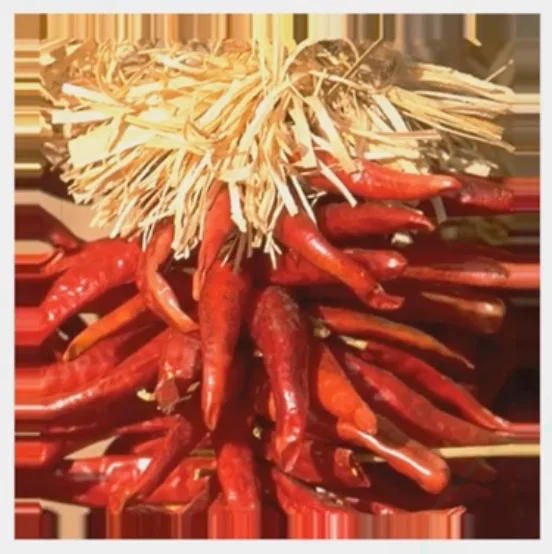
What is texture?
- Regular or stochastic patterns caused by bumps, grooves, and markings
- We can represent textures by computing responses of different filters
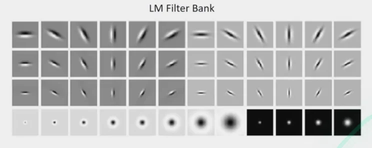
Filter Bank
- Process image with each filter and keep resposnes
- for example, sum of the responses may be stored to tell how strongly the image responds the filter
- Measure responses of blobs and edges at various orientations and scales
- Record simple stats of absolute filter responses