2.1 Frequency
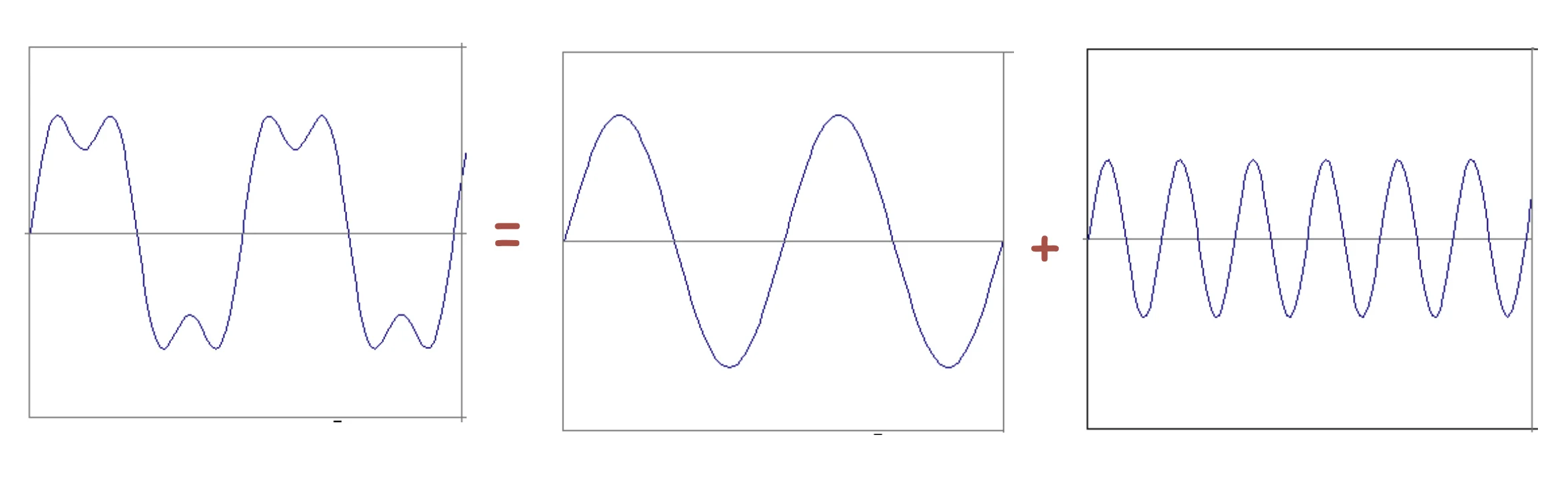
A sum of sines
Building blocks:
Frequency Spectra
Example
How to construct a square wave
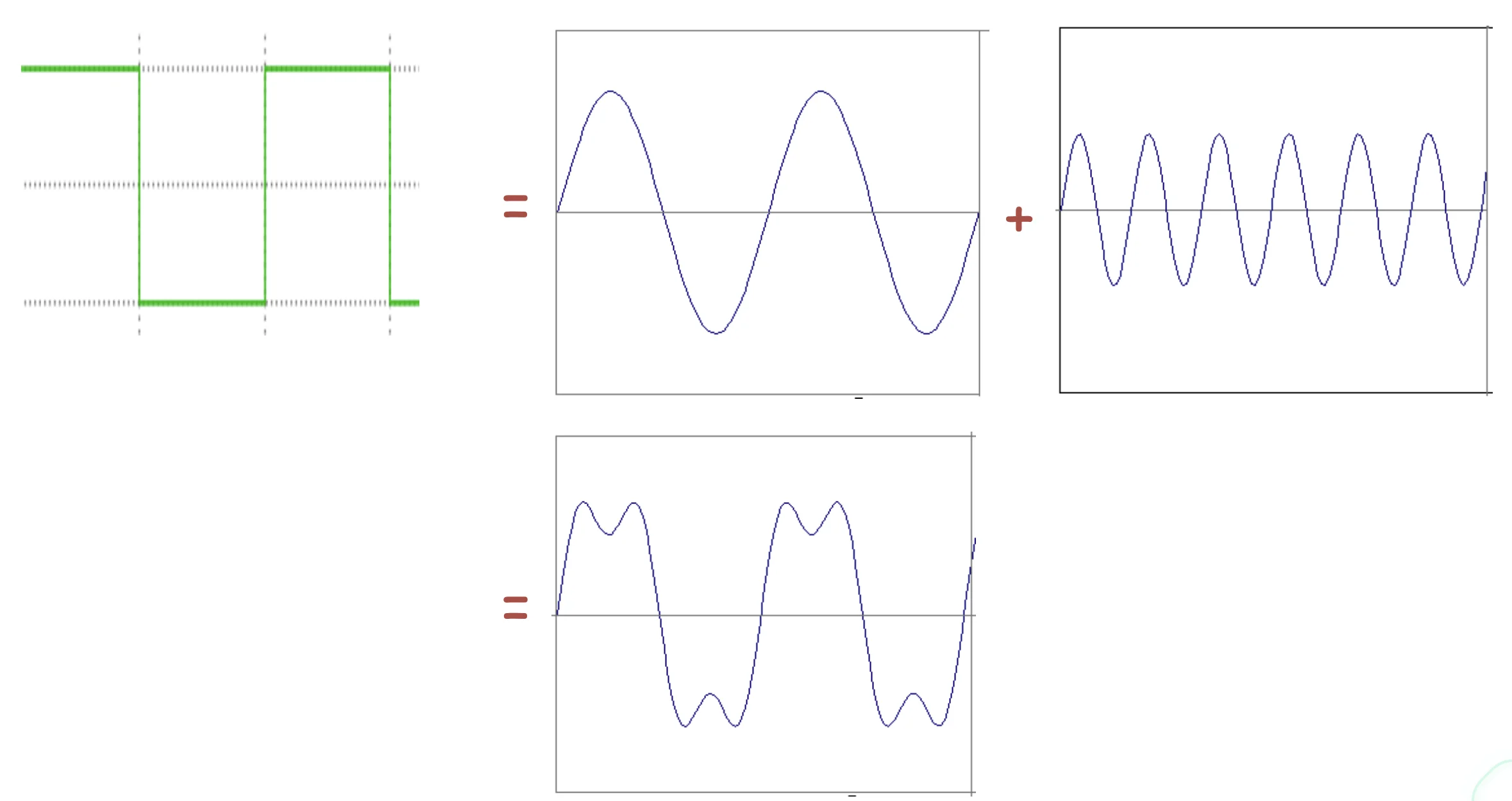
- Add enough of these signals
at decreasing amplitudesas youincreasethefrequencyof this sinusoid. Then, the sum of signals converges to asquare wave
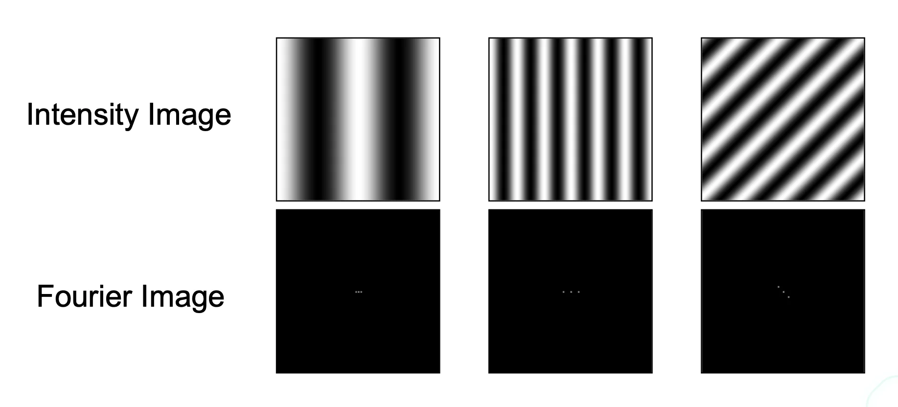
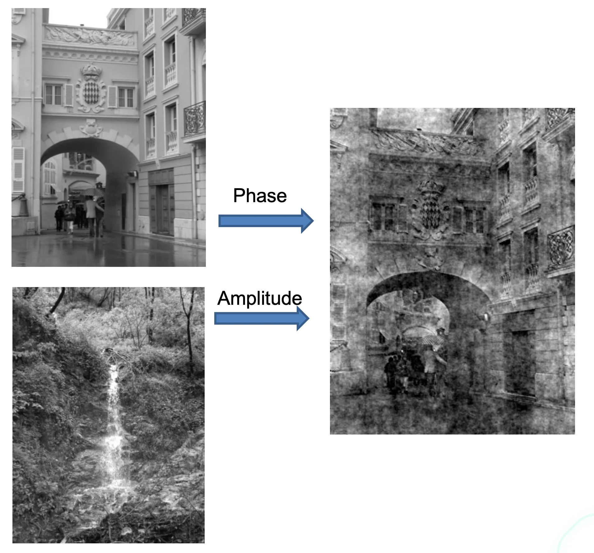
Fourier Analysis in Images
Fourier Transform
-
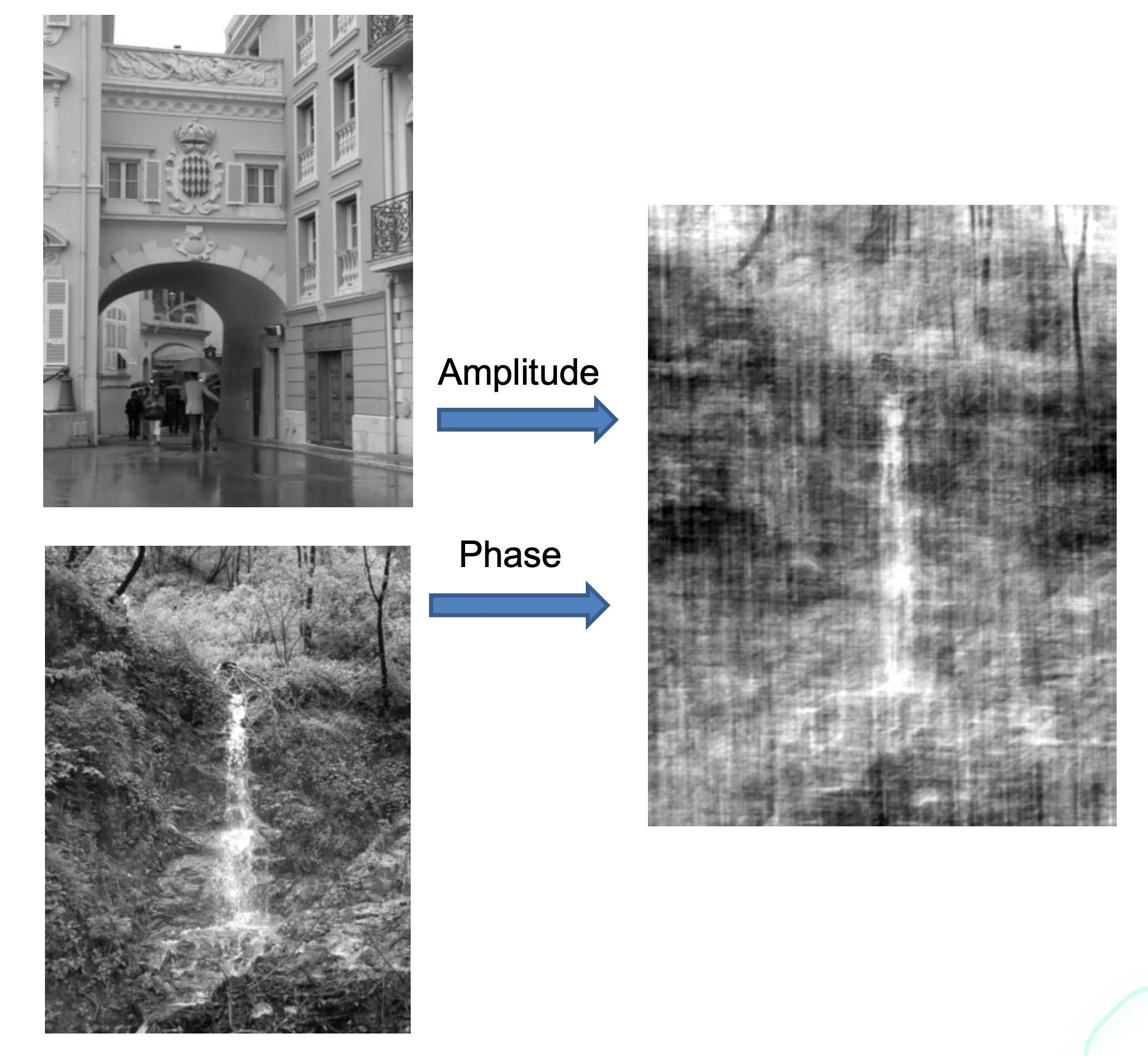
Fourier transform stores the
amplitudeandphaseateach frequency -
Amplitude: encodes the number of signals at a particular frequency -
Phase: encodes spatial information
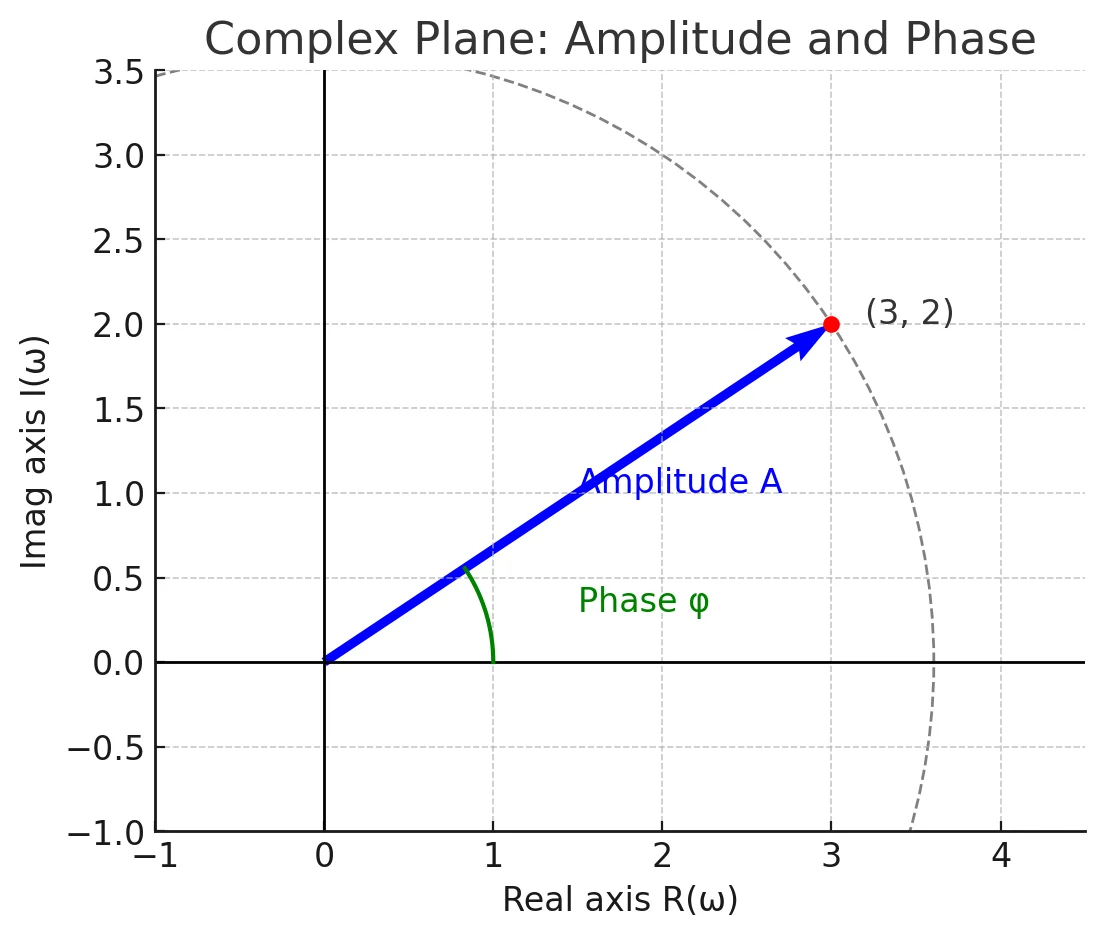
1. Amplitude Formula
where:
-
: the real part of a complex function (often a Fourier transform).
-
: the imaginary part.
-
: a complex number representing a signal at frequency .
Amplitude on Cosine Wave
# Time vector
t = np.linspace(0, 2*np.pi, 500)

# Parameters
omega = 1.0 # frequency
phi = np.pi/4 # fixed phase

# Different amplitudes
A1 = 0.5
A2 = 1.0
A3 = 1.5

# Signals
y1 = A1 * np.cos(omega*t + phi)
y2 = A2 * np.cos(omega*t + phi)
y3 = A3 * np.cos(omega*t + phi)

# Plot
plt.figure(figsize=(8,5))
plt.plot(t, y1, label=r'$A = 0.5$', linewidth=2)
plt.plot(t, y2, label=r'$A = 1.0$', linewidth=2)
plt.plot(t, y3, label=r'$A = 1.5$', linewidth=2)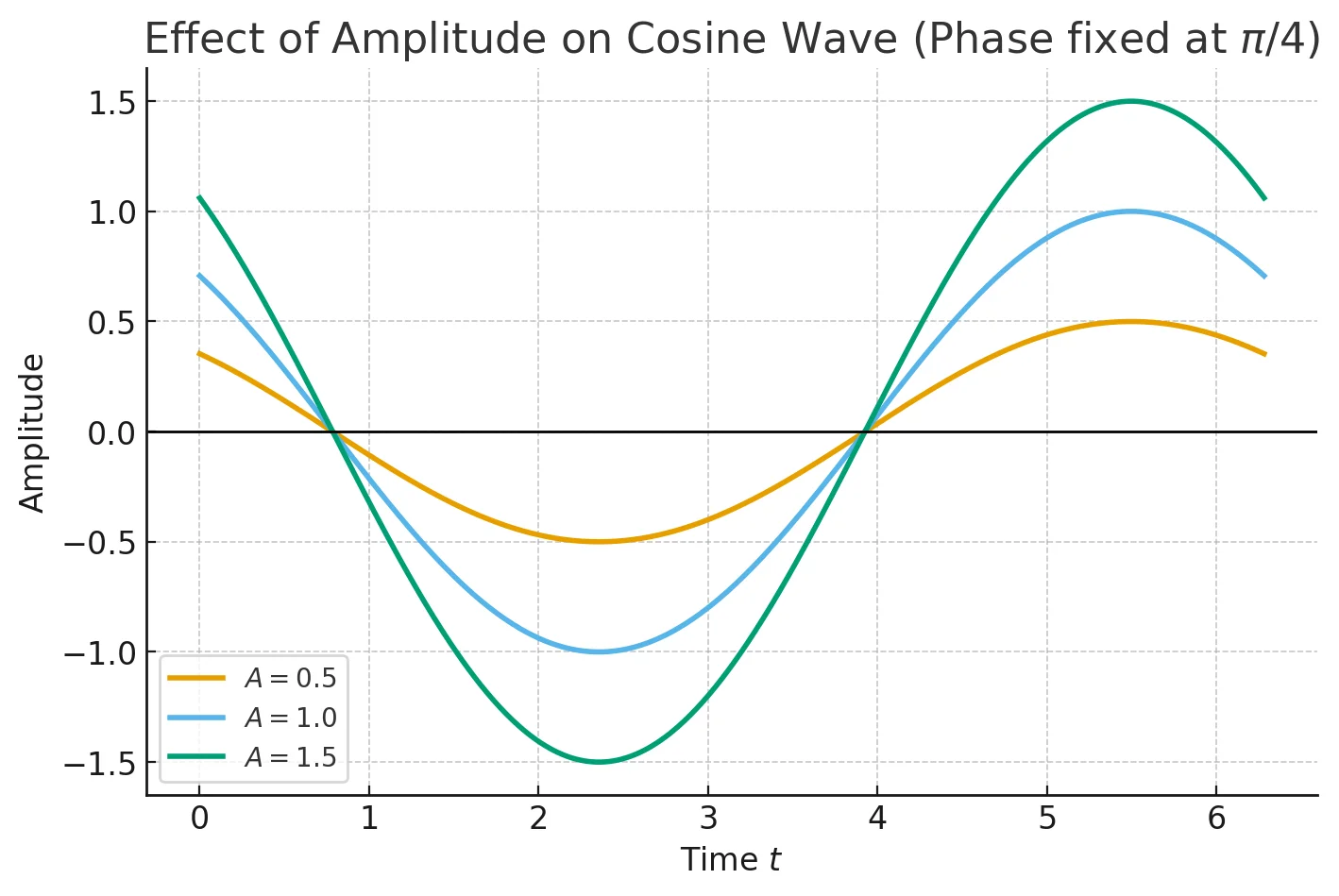
Note
The amplitude (or magnitude) is just the length of this complex number in the complex plane. Pythagorean theorem:
2. Phase Formula
-
The phase angle describes how much the sinusoidal signal is shifted horizontally relative to a cosine (or sine).
-
In the complex plane, the phase is the angle made by vector with the positive real axis.
Shift on Cosine Wave
# Time vector
t = np.linspace(0, 2*np.pi, 500)

# Parameters
A = 1.0 # amplitude
omega = 1.0 # frequency

# Different phases
phi1 = 0
phi2 = np.pi/4 # 45 degrees
phi3 = np.pi/2 # 90 degrees

# Signals
y1 = A * np.cos(omega*t + phi1)
y2 = A * np.cos(omega*t + phi2)
y3 = A * np.cos(omega*t + phi3)

# Plot
plt.figure(figsize=(8,5))
plt.plot(t, y1, label=r'$\phi = 0$', linewidth=2)
plt.plot(t, y2, label=r'$\phi = \pi/4$', linewidth=2)
plt.plot(t, y3, label=r'$\phi = \pi/2$', linewidth=2)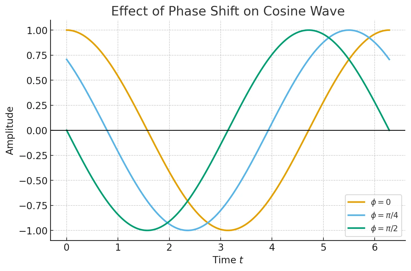
Note
In practice, we often use atan2(I, R) instead of, because atan2 takes into account which quadrant the point lies in (avoiding sign ambiguities).
3. Euler’s Formula
-
Exponentials with imaginary exponents represent rotations in the complex plane.
-
The real part gives a
cosine, and the imaginary part gives asine.
So when we write:
-
: the amplitude (the radius in the complex plane),
-
: the phase (the angle).
Tip
The derivation is shown in Euler’s Formula
Integration and Fourier Transform
Important
Imaginary number is presented with due to mathematical convention
General Form
- : Fourier Transform
- : frequency domain
Continuous Fourier Transform (CFT)
used when is a continuous signal
- projects the singal onto complex exponentials
- At each frequency , it computes the amount of that frequency is present in the singal
Discrete Fourier Transform (DFT)
used when is a discrete signal
where:
- : the number of samples
- : frequency index (integer)
- cycles through different frequencies, checking how much of each frequency is present
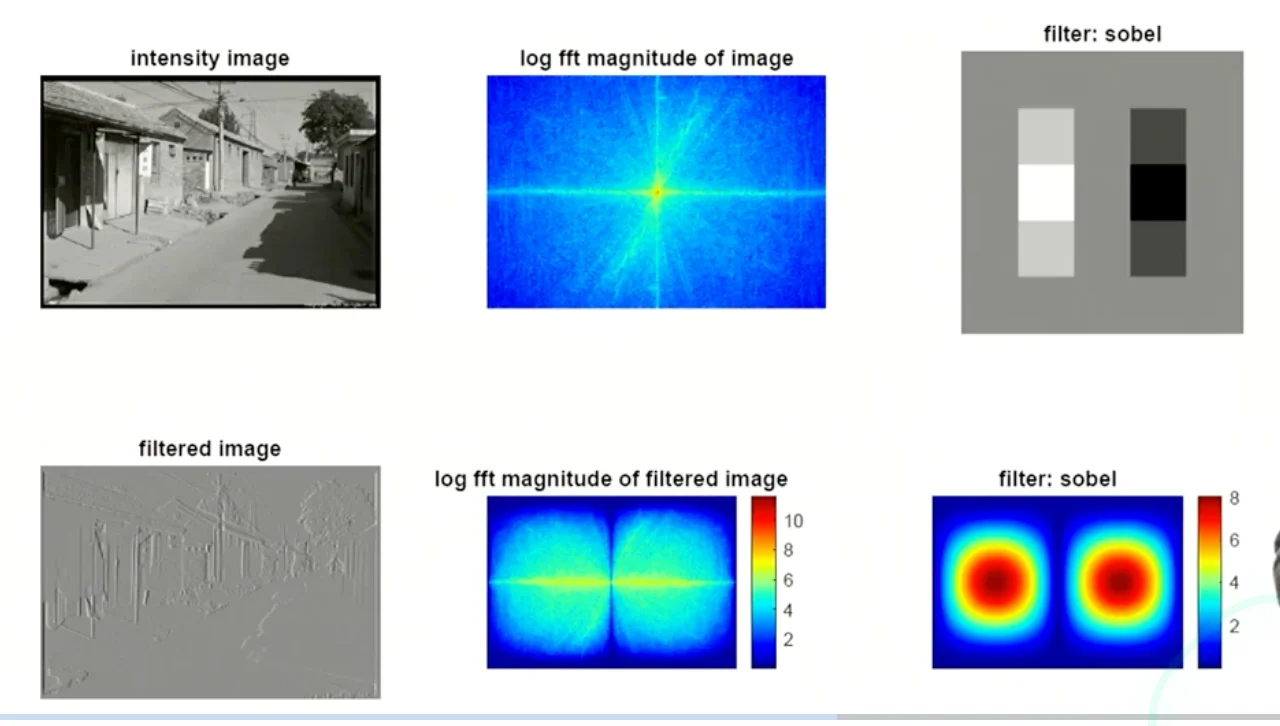
The Convolution Theorem
- The Fourier transform of the convolution of two functions is the same as the product of their Fourier transforms
- The inverse Fourier transform of the product of two Fourier transforms is the convolution of the two inverse Fourier transforms
Important
- Convolution in the spatial domain is the same as the Multiplication in the frequency domain
- FFT (Fast Fourier Transform) can convert between the spatial domain and frequency domain in with being the number of pixels
Properties of Fourier Transform
- Linearity
- Fourier transform of a real signal is symmetric about the origin
- The energy of the signal is the same as the energy of its Fourier transform
- You don’t lose information when you convert back and forth between spatial and frequency domains
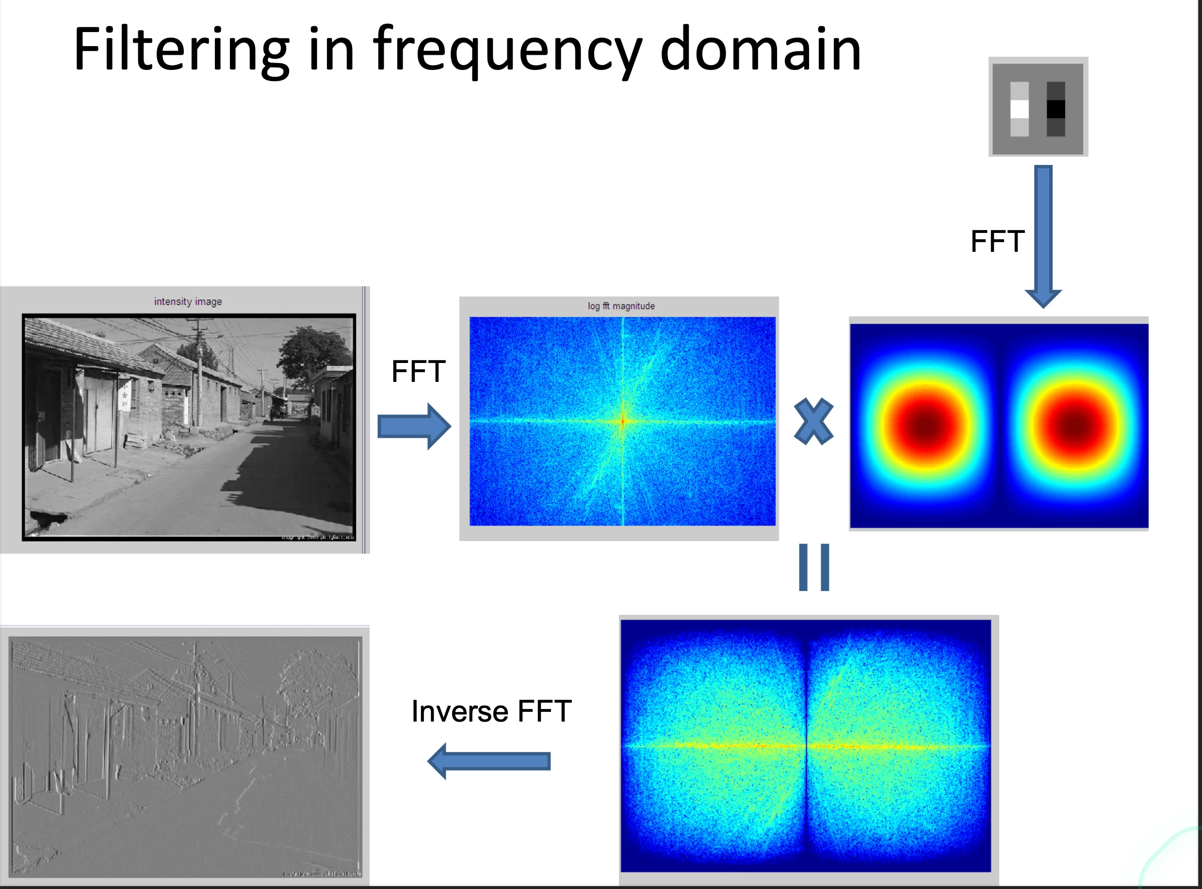
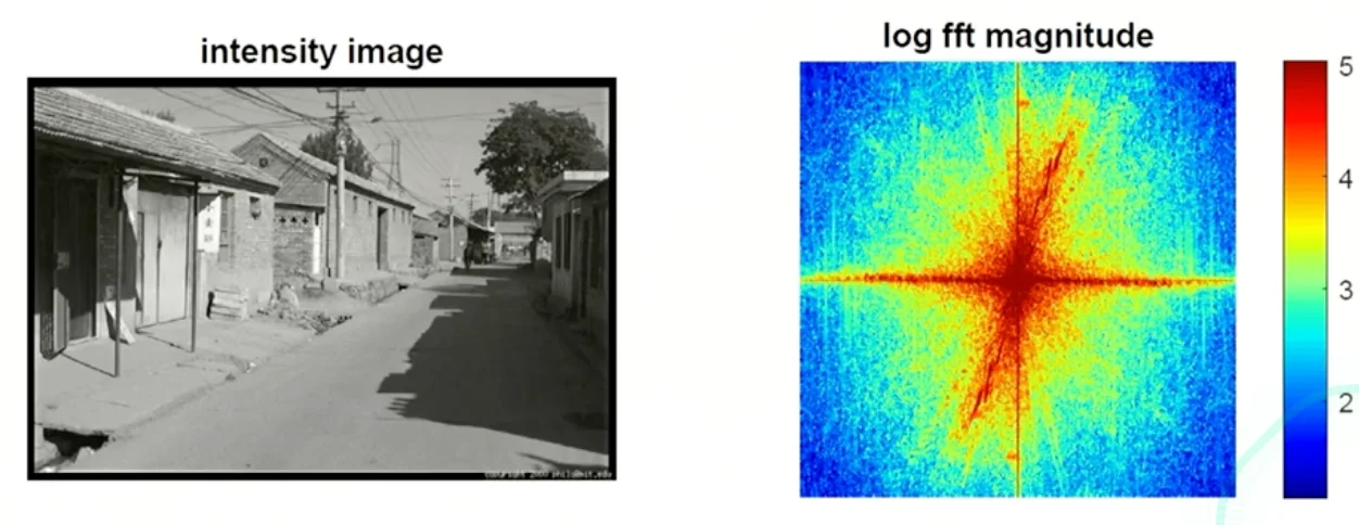
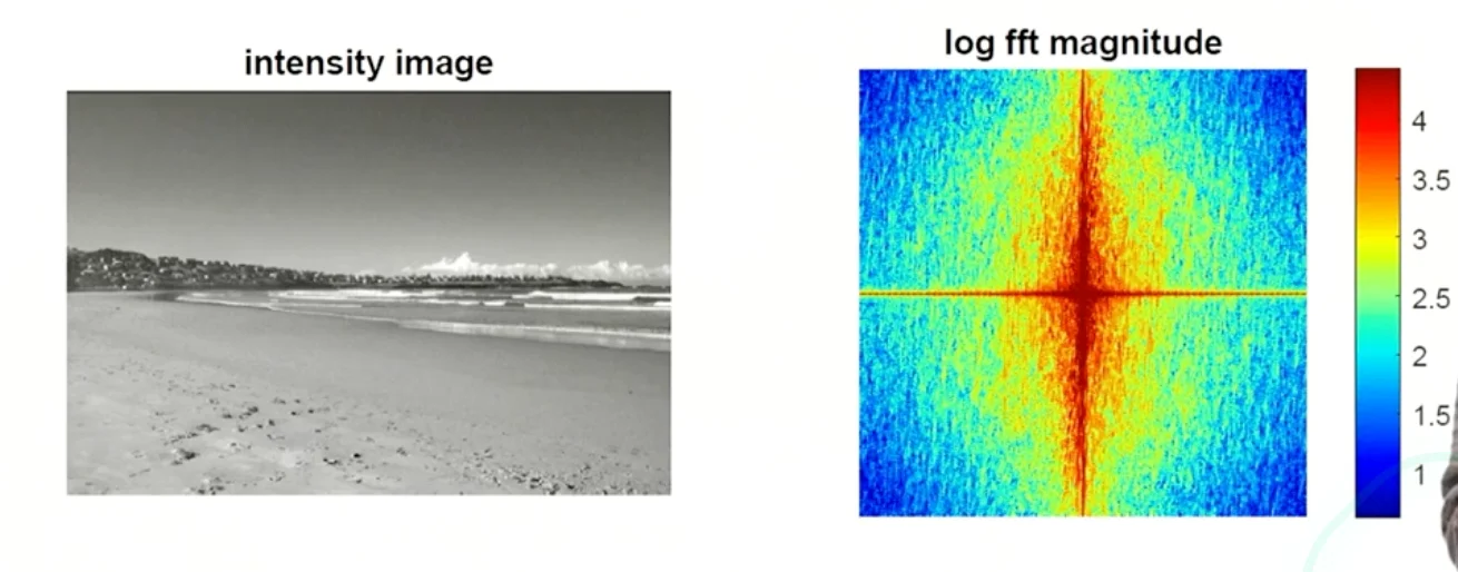
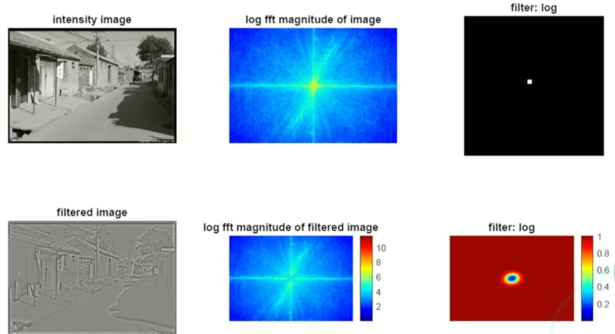
Image Frequency Examples
- Frequency changes
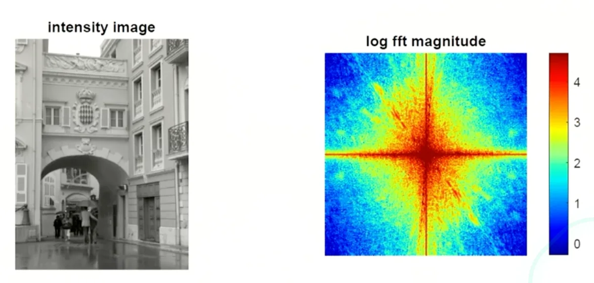
- Moving horizontally and vertically crosses a lot of edges.
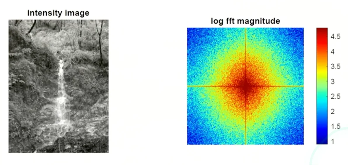
- Frequencies are spread evrywhere more rounded
Note
For city images it’s more common to have star shapes, while natural images are tend to be rounded shapes.
Comparison of filters
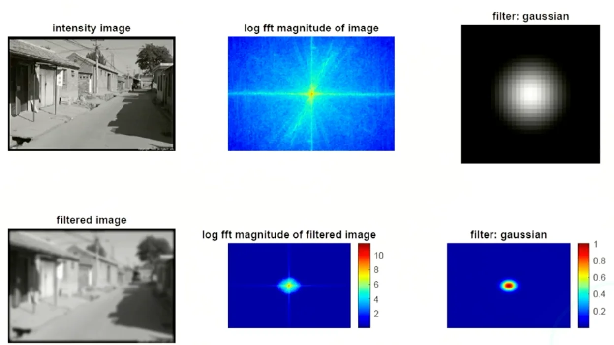
- Gaussian filter selecting for lower frequencies
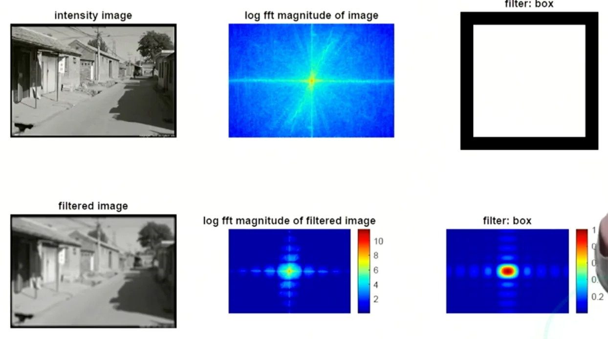
- Box filter:
- preserve both low and high frequencies
- The disjointed range of higher frequencies is also preserved, so it doesn’t prove as good of a smoothing effect as a Gaussian
Mixing Images
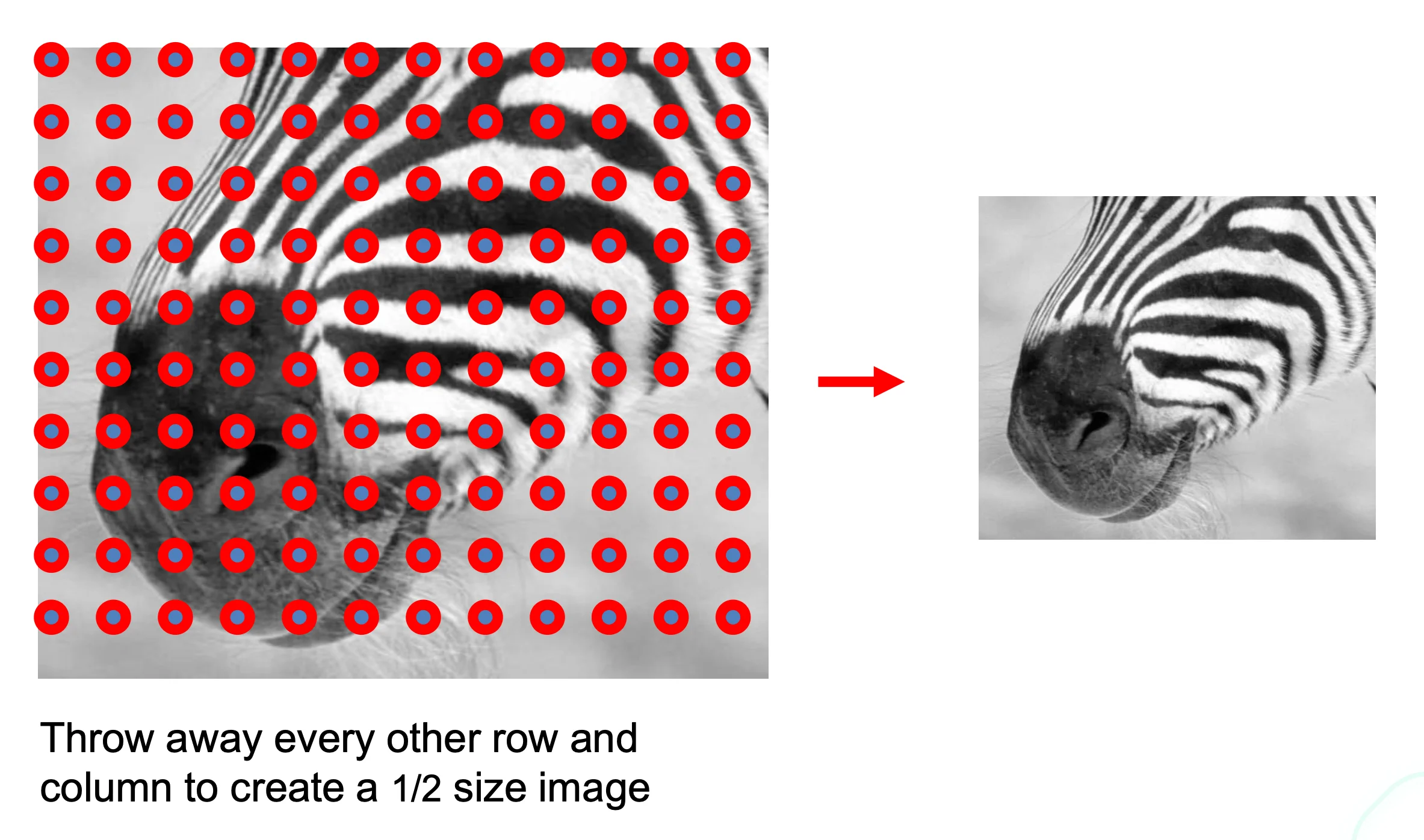
Sampling
- Why does a lower resolution image still make sense to use?
- Images are typically smooth, and sampling cuts off high frequencies, which are not that many in a image
- We can thus shrink an image without losing a lot of information
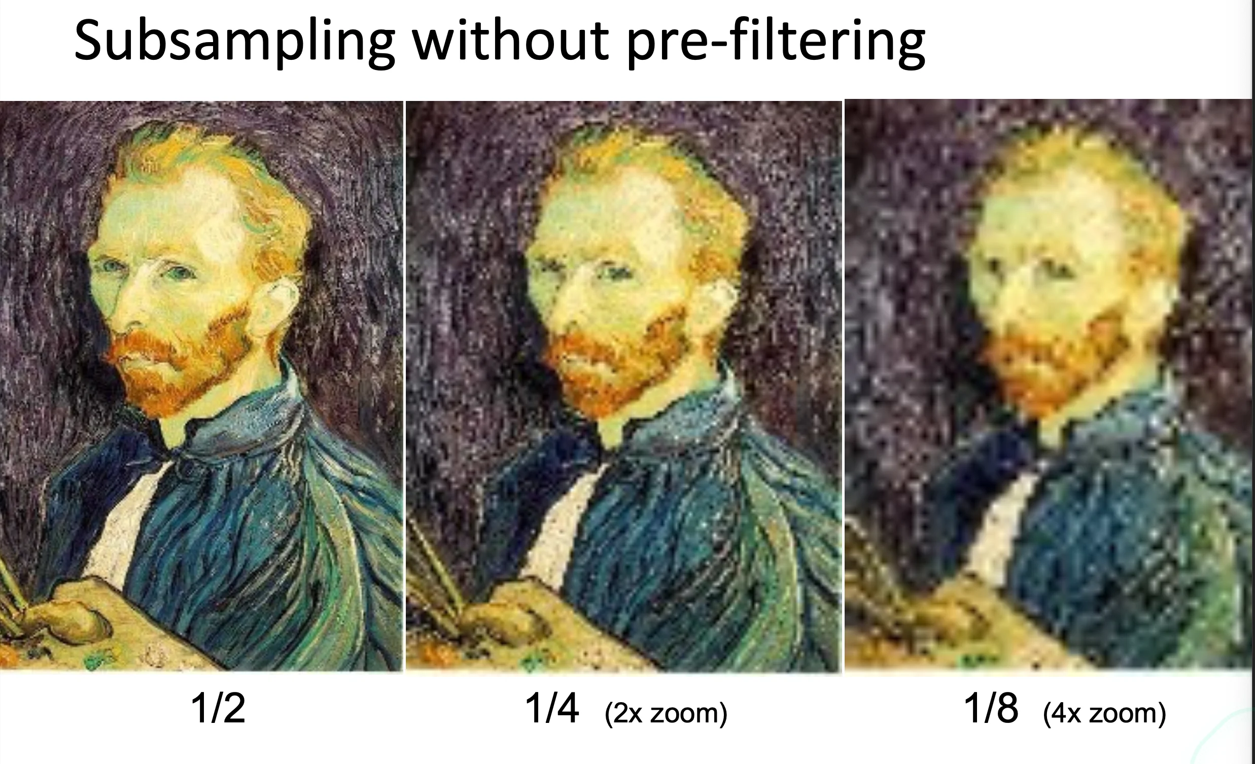
Aliasing Problem
- Sub-sampling may be dangerous as characteristic errors may appear
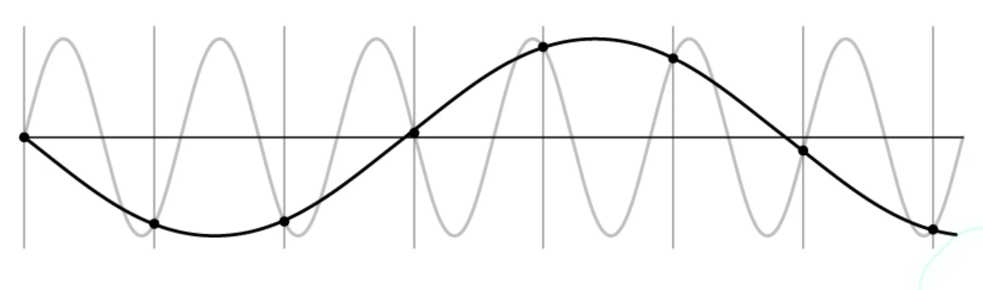
- We create an artifact that’s not in the original signal
Nyquist-Shannon Sampling Theorem
- When sampling a signal at discrete intervals, the sampling frequency must be
- : max frequency of the input signal
- This allows a reconstruction of the original image
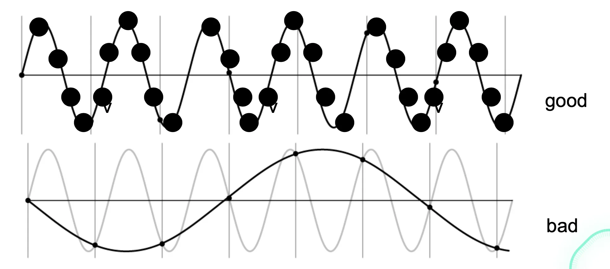
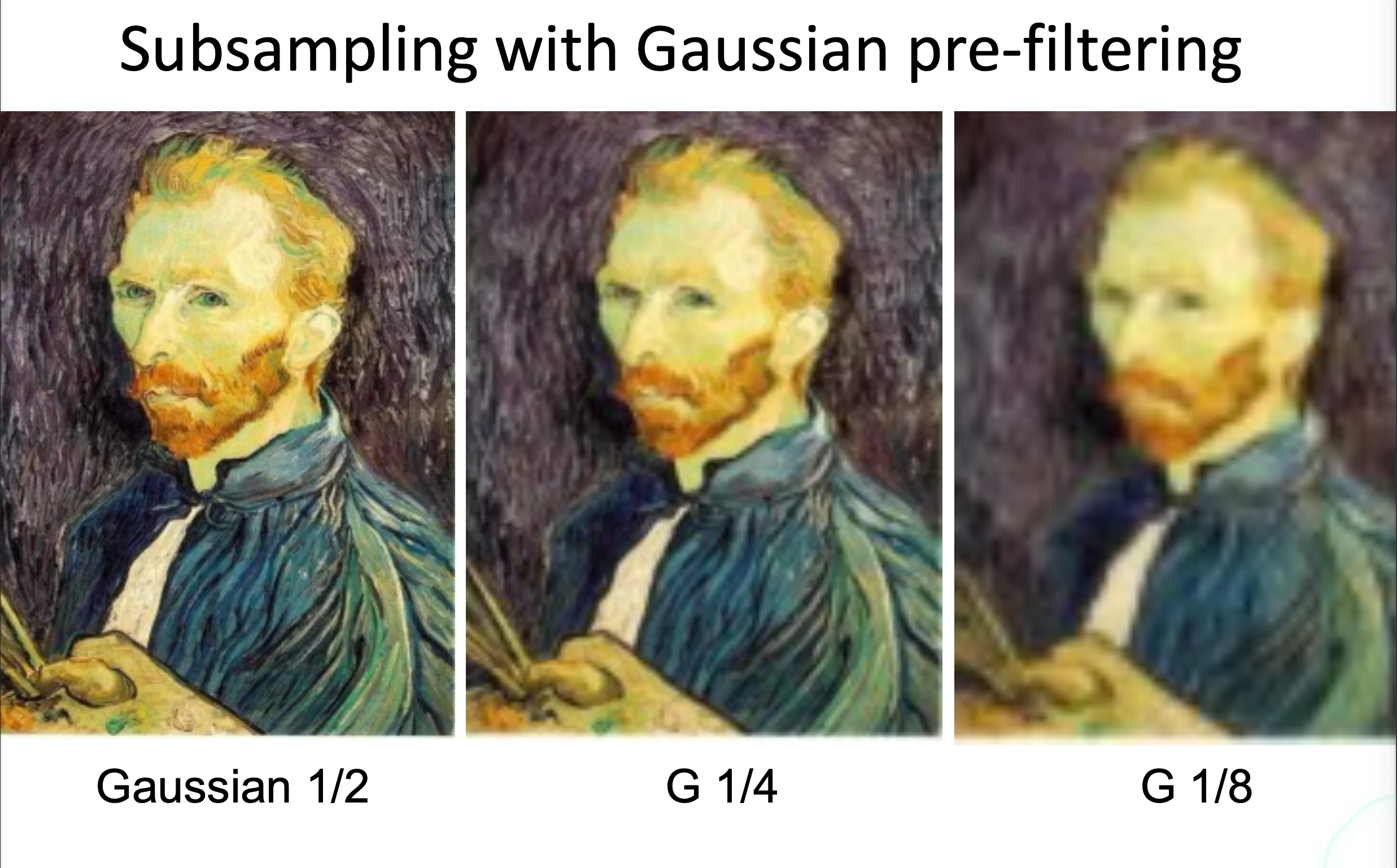
Solution (Anti-aliasing)
- Sample more often
- Get rid of all frequencies that are greater than half of the new sampling frequencies
- lose some high frequencies information but it’s better than aliasing
import numpy as np
from scipy.ndimage import gaussian_filter

# 1. Start with image(h, w)
# Let's assume `image` is a NumPy array of shape (h, w)

# 2. Apply low-pass filter (Gaussian blur)
im_blur = gaussian_filter(image, sigma=1) # fspecial('gaussian', 7, 1) ≈ Gaussian with σ=1

# 3. Sample every other pixel
im_small = im_blur[::2,::2]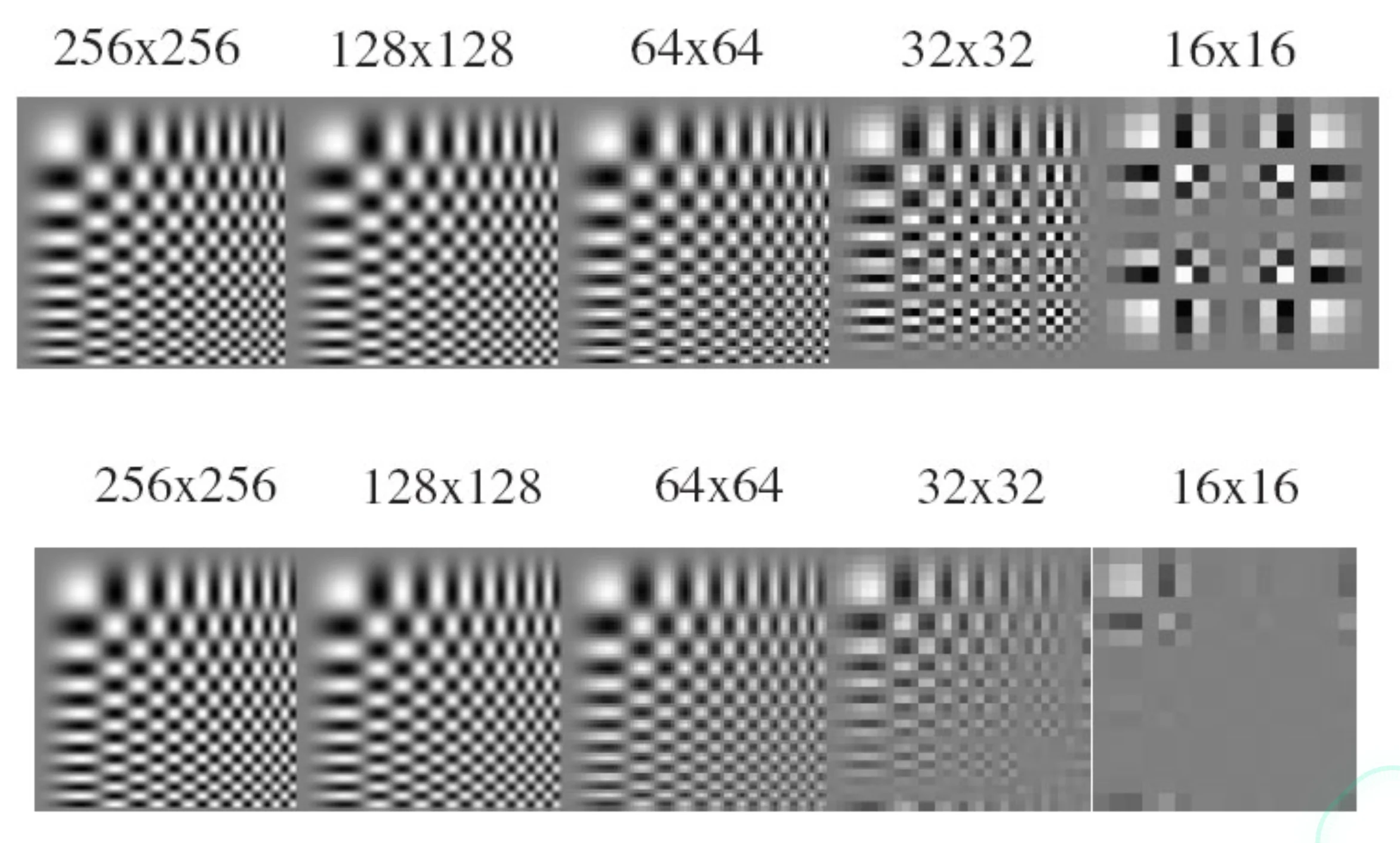
Hybrid Image in FFT
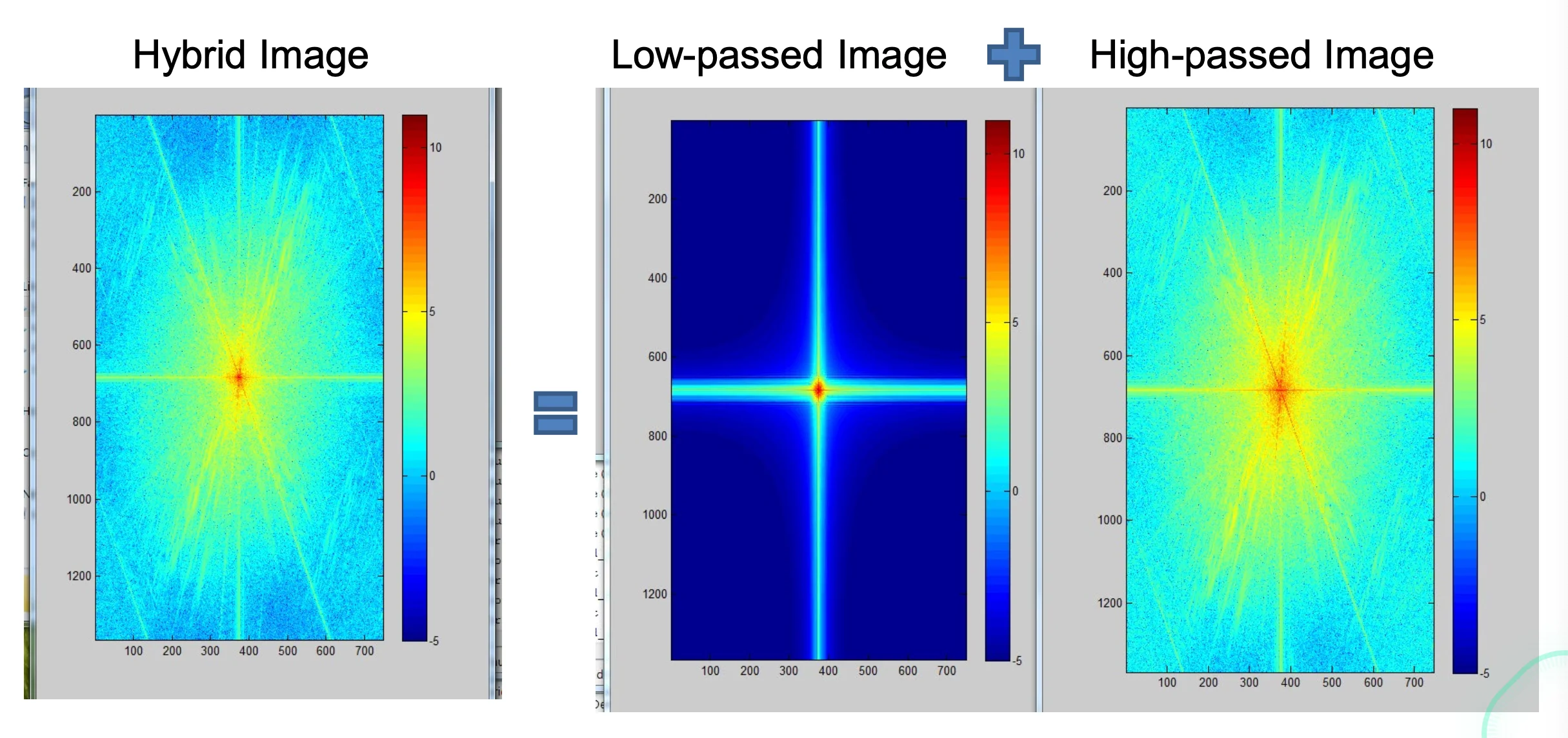
- When we’re close to the image, the higher frequencies dominate our perception, so we observe them much more readily
- When we’re further away, high frequencies are smoothed out and we can only observe the low passed image