2.2 Template Matching
Review - Matching Frequency Plots to Images
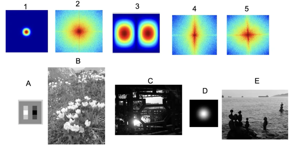
- A lot of horizontal edges due to the waves and due to their horizons.
- There aren’t a lot of vertical edges
Template Matching
- Goal: find an eye in image
- Challenge:
- What is a good similarity or distance measure between two patches?
- Correlation
- Zero-mean correlation
- Sum Square Difference
- Normalized Cross Correlation
Important
- Assume the following formulas are formulated given that:
- : image
- : filter
Correlation
- Filter the image with eye patch
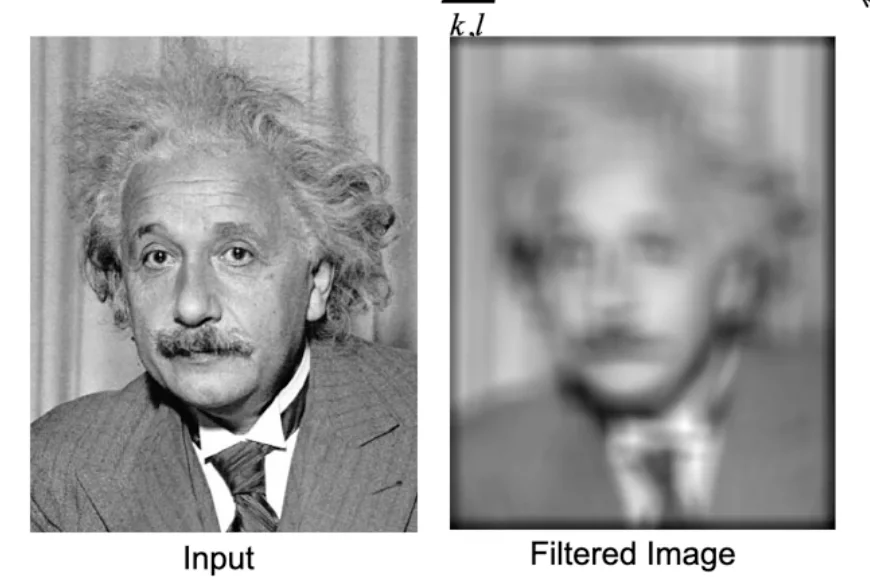
- = image
- = filter
Warning
This simply takes weighted summation over each position of the image
- Places that are dark lowest possible response
- Places that are white highest possible response
Zero-mean correlation
- Simple fix for correlation
- Instead of scanning with the direct intensity patch, we subtract the average intensity from the template
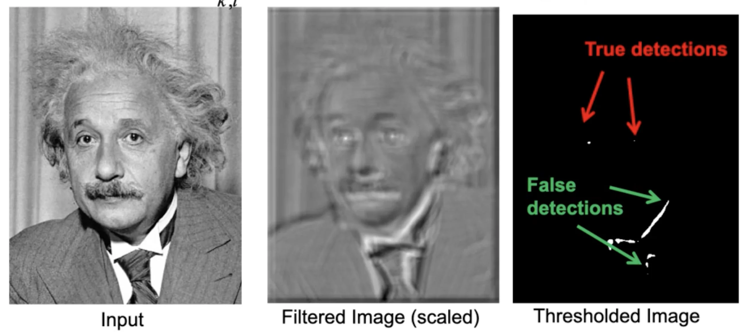
- : mean of f
- If patch and templates are dark in the same places and light in the same places, you’re going to have a strong positive response.
Warning
The method only cares about whether a pixel is bright or dark in the same places, but it doesn’t take the degrees into considerations
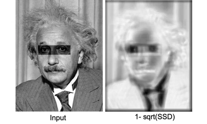
Sum of Squared Difference (SSD)
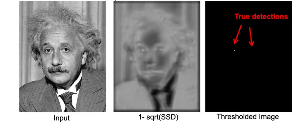
- Take the template and scan it over the image.
- At each position you take the
differencebetweenthe corresponding pixels in the templateandimage patch.
Tip
SSD enforces that the intensities have to be exactly the same as the image in the template
Implement SSD with linear filter
Warning
- SSD requires you have the exact matching of intensities.
- The change of contrast would lead to the Failure of template matching
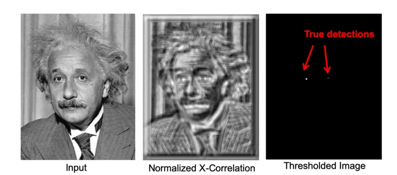
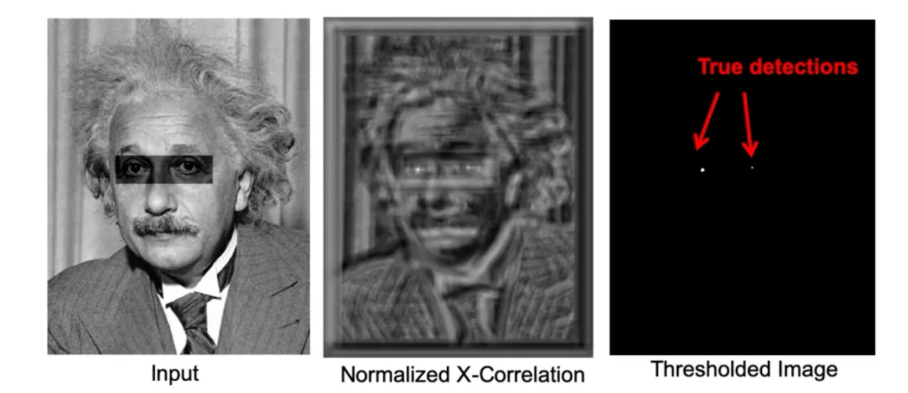
Normalized Cross-correlation
- By doing this, the multiplicative factor induced by image scaling will be cancelled out by the standard deviation.
Tip
- You can also do a simple cross-correlation without normalizing it (not dividing standard deviation).
- This works when you only care about the issues related to the shifts of intensity without dealing with the contrast and multiplications of intensity
Without Scaling
With Scaling
Tip
All these template matching methods are implemented with cv2.matchTemplate(im, template, cv2.TM_CCOEFF_NORMED) with the difference of the third argument.
Summary of Different Matching Filter
Zero-mean filter: Fastest but not a great matcherSSD: Next fastest, sensitive to overall intensityNormalized coss-correlation: Slowest, invariant to local average intensity and contrast
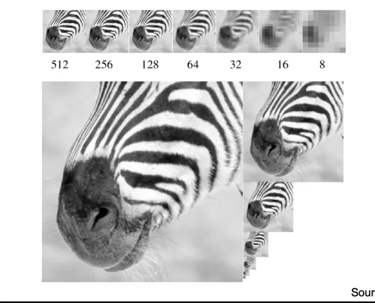
Sampling
Gaussian Pyramid
- Repeatly perform
Image -(Gaussian Filter)-> Low-pass Filtered Image -(Sample)-> Low-Res Image
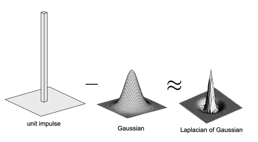
Laplacian pyramid
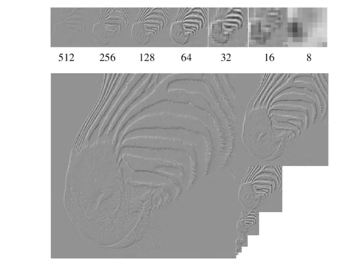
Laplacian Filter
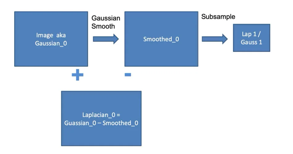
Computation Process
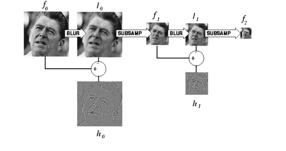
- Apply Gaussian filter to the image
- Subtract the smoothed images from the original image
- Down-sample
Warning
You can reconstruct the image from Laplacian pyramid but you may lose some information
Lossless Reconstruction
Original Process
A small tweak
- Instead of
just smoothingandsubtractingthe smoothed from the original, we:
- Compute the Lap1
- up-sample it
- smooth it
- subtract that result from the image to get the top level of a Laplacian pyramid
Hybrid Image in Laplacian Pyramid
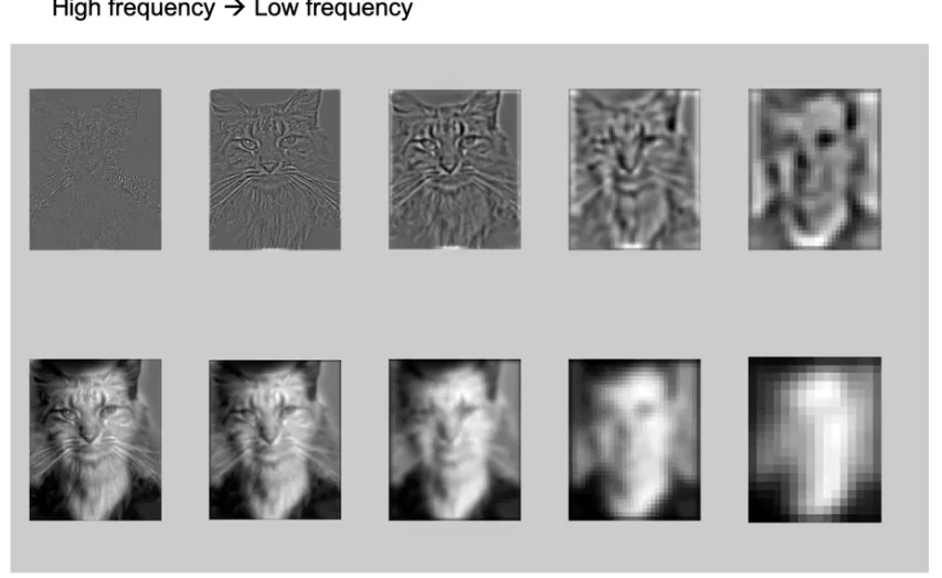
- In the high frequency, only the cat is visible (Laplacian Smoothing)
- In low frequency, humans are more visible (Gaussian Smoothing)
Coarse-to-Fine Search
1. Start at the coarsest pyramid level
- Search the full range of translations
- Find the best translation
2. Upsample the estimate when moving to the next finer level
Note
Image size doubles between levels
3. Local Refinement
- Instead of searching the full range again, only serach a small window:
4. Repeat until reaching the original resolution
Image Registration
Aligning two images of the same scene so that corresponding points overlap
where:
- is the translation vector we want to estimate.
Image Pyramid
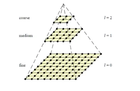
- Build an image pyramid
level 0: full-resolution image, sizelevel 1: downsampled by factorlevel 2: downsampled by again- This gives progressively smaller, blurrier images that retain coarse structure but lose higyh-frequency detail
Sum of Squared Difference (SSD) Matching
Evaluate how well two images align under translation
- Compute SSD for each candidate translation from
coarse to fine
- Choose the translation that minimizes
Tip
Corase-to-fine image registration is faster to compute as at each coarse level, images are much smaller and there are few pixels to compare.
Caution
- Not Guaranteed Optimal
- If the corase-level images lose too much detail, the algorithm may converge to the wrong translation.
- Works in practice
- Meaningful structure is in low frequencies
- Noice is reduced at coarse scales
- Danger
- Overly downsampling may lead to the inability to align images correctly