2.3 Denoising, Compression
Image Alignment with FFT
- can be used to efficiently implement
Recap of Convolution Theorem
- : convolution in the spatial domain
- :Fourier transform in the frequency domain
SSD Implementatioon with FFT
Standard SSD Formula:
- : The larget
imageor scenein whichyou’re searching - : The smaller
image patchor patternthatyou’re finding - : The offset from the original position
[!IMPORTANT] > Computational Complexity
- Spatial Domain SSD:
- is image size
- is template size
- FFT-based SSD
Image Compression Principle
- Most intensity information is concentrated in lower frequencies
JPEG Compression (lossy)
- JPEG is a lossy compression method that exploits the human visual system’s reduced sensitivityto high-frequency changes and chrominance variations
1. Color Space Conversion
- Convert to
2. Sub sample Chroma by factor of 2
- Subsample and channels by factor of 2
- People are not sensitive to color
3. Block Decomposition
- Divide each channel into pixel blocks
- Subtract 128 from each pixel (center around 0 for better compression)
4. Discrete Cosine Transform (DCT)
- : DC component (average intensity)
- : Highest horizontal frequency
- : Highest vertical frequency
- : Highest diagonal frequency
where:
5. Quantization
- is the quantization table value at position
- A typical quantization table:
16 11 10 16 24 40 51 61
12 12 14 19 26 58 60 55
14 13 16 24 40 57 69 56
14 17 22 29 51 87 80 62
18 22 37 56 68 109 103 77
24 35 55 64 81 104 113 92
49 64 78 87 103 121 120 101
72 92 95 98 112 100 103 99
6. Entropy Encoding
- Use Huffman coding to encode quantized coefficients
- Zigzag scanning to group zeros together
- Run-length encoding for sequences of zeros
JPEG Reconstruction
1. Dequantization
2. Inverse DCT
Caution
JPEG Artifacts
- Blcoking: 8x8 block boundaries become visible at high compression
- Ringing: Oscillations near sharp edges due to quantization of high frequencies
- Color bleeding: Chroma subsampling causes color information to spread
PNG (Lossless)
- Predict that a pixel’s value based on its upper-left neighborhood
- Store difference of predicted and actual value
- Pkzip it (DEFLATE Algorithm)
Important
- PNG exploits image smoothness by predicting each pixel from its neighbors and storing ONLY the prediction errors.
- It’s the best for images with few colors, sharp edges, text, graphics
Denoising
Reducing Gaussian Noises
- Smooth out the noises by applying Gaussian filter
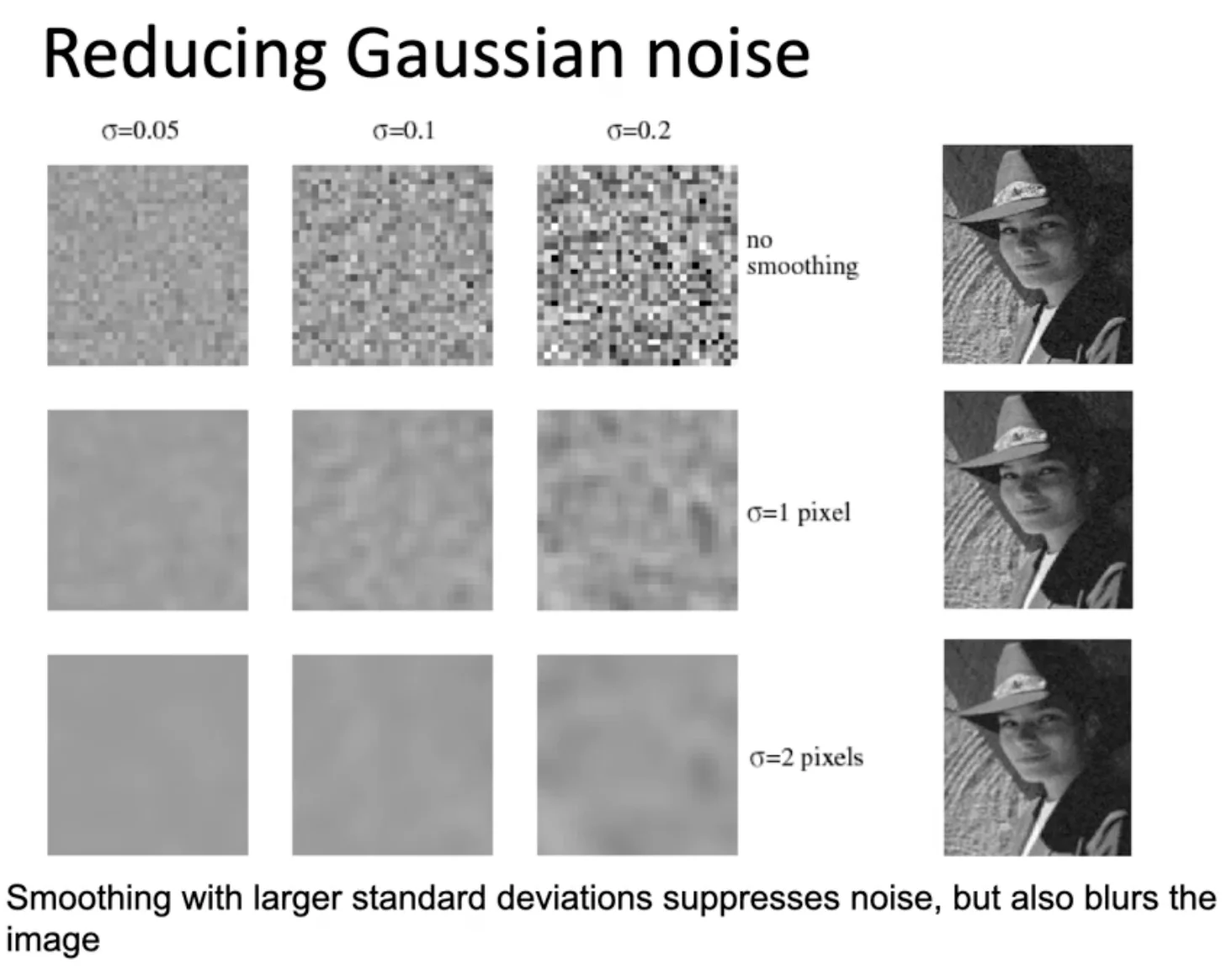
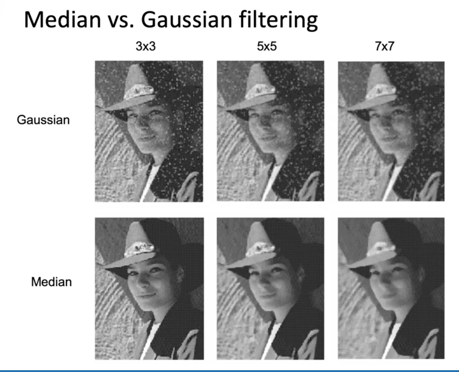
Caution
Gaussian filtering may induce salt-and-pepper Noises
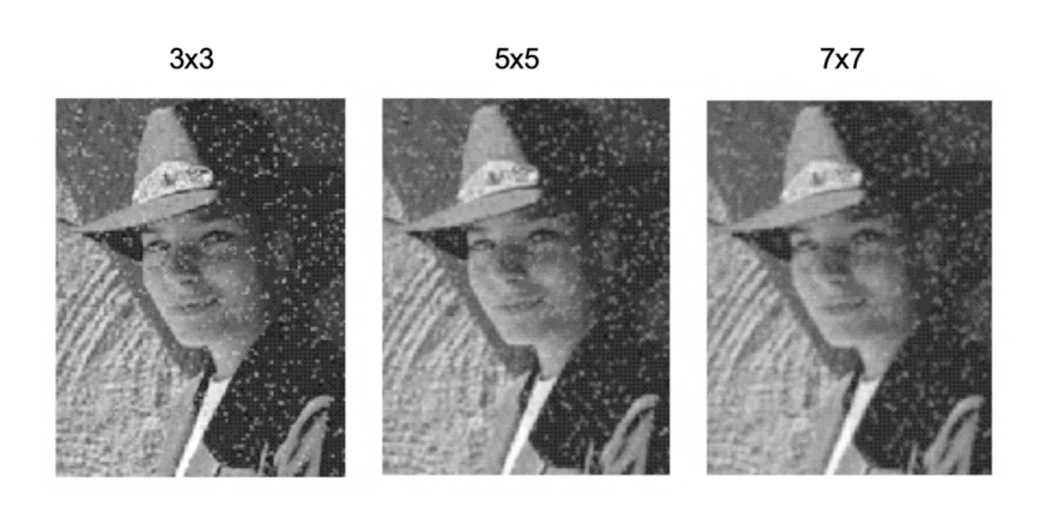
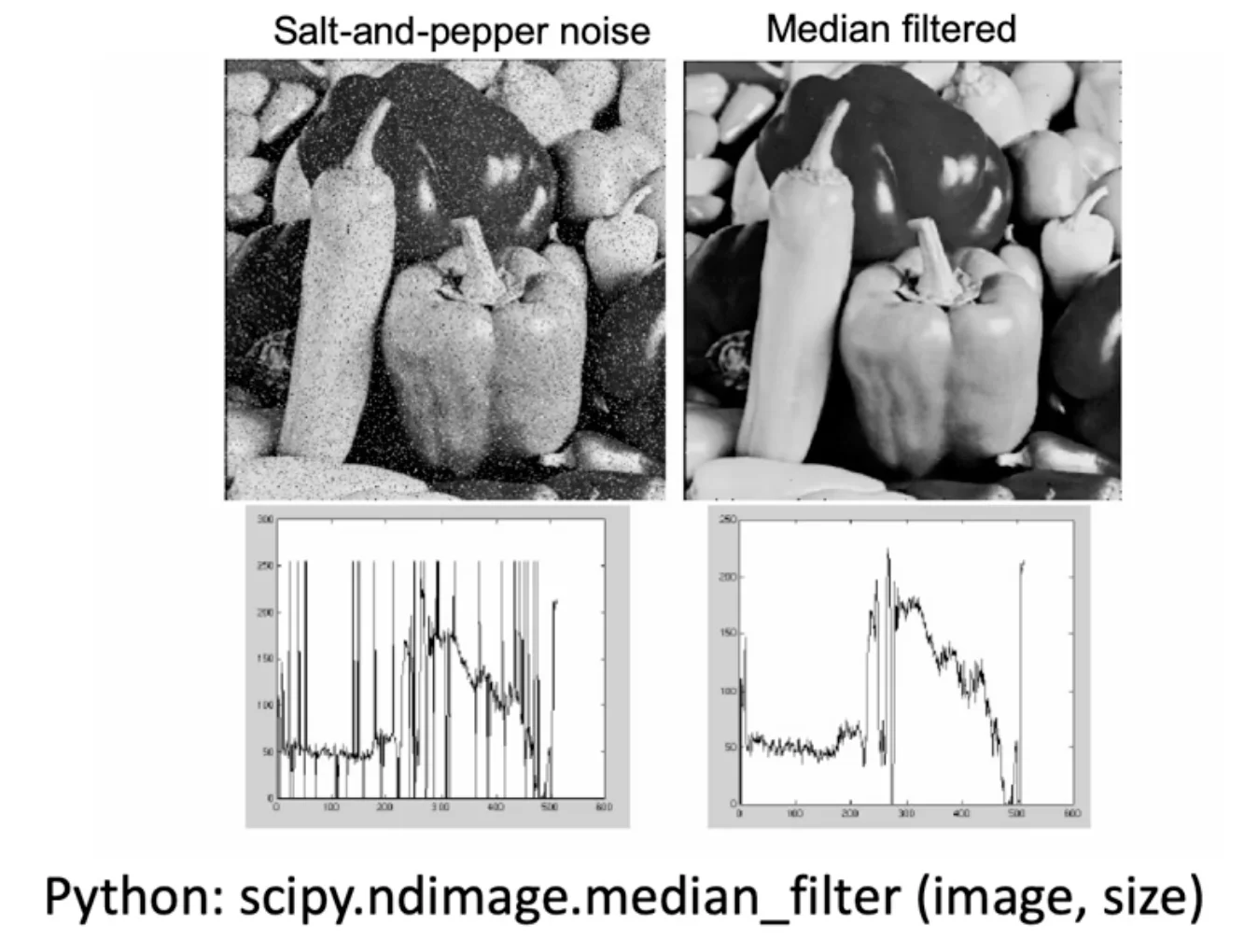
Median Filtering
- Median filtering is robust to outliers
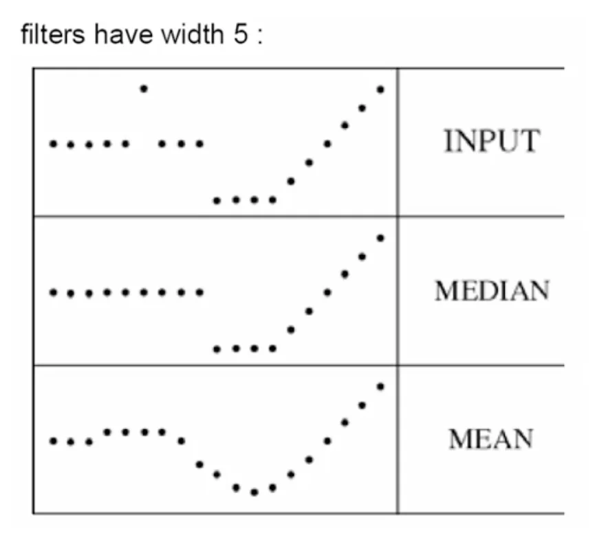
Median vs Gaussian
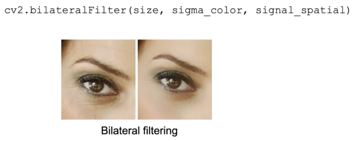
Bilateral Filtering (weight by spatial distance and intensity difference)