3.2.3 Histogram Equalization
Histogram Equalization
- Reassign values so that the number of pixels with each values is more evenly distributed
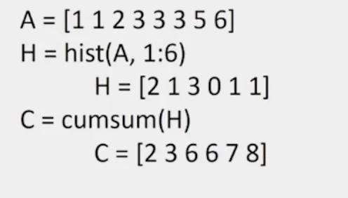
Histogram
- a count of how many pixels with the same value
Cumulative histogram
- a count of number of pixels less than or equal to each value
Example
Histogram Equalization
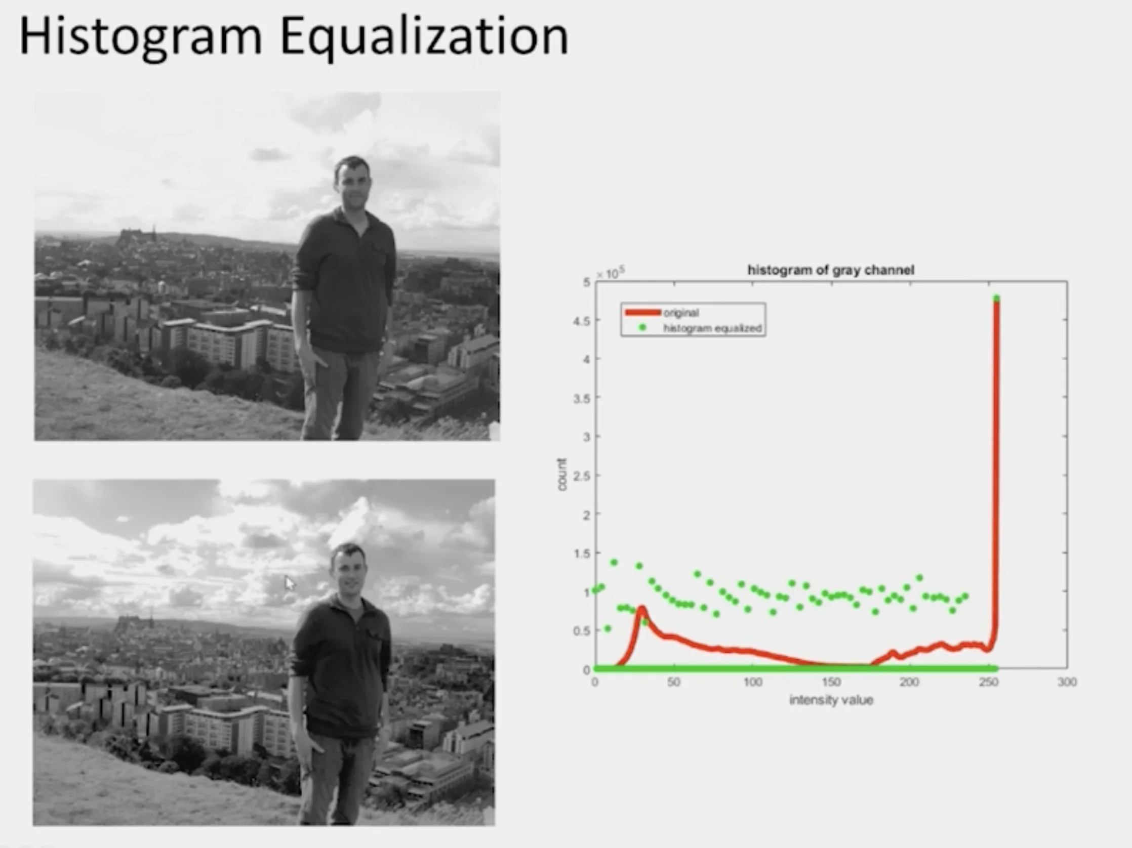
- The original intensity is culstered on the left and right sides.
- After the equalization, the values are more evenly distributed.
Algorithm
- Given image with pixel values
- Compute cumulative histogram
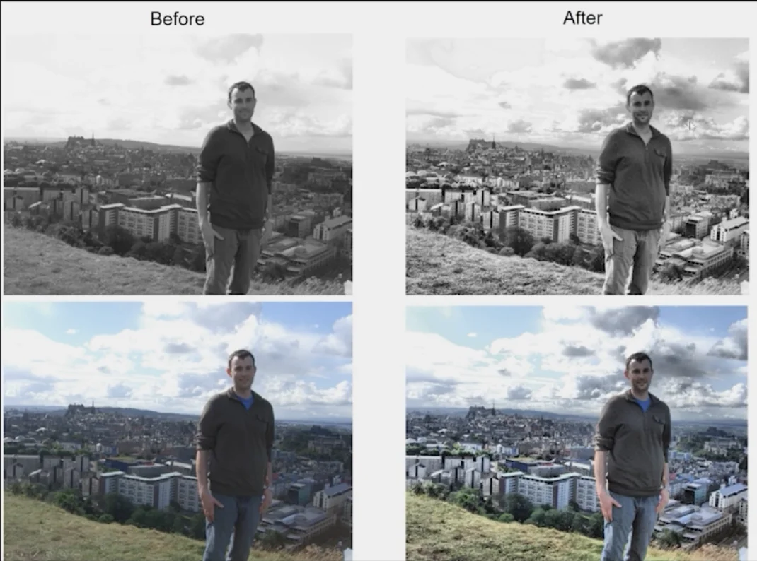
- Blends between original image and image with equalized histogram
- balancing factor
- the percentile of the pixel
Locally weighted histograms
- Compute cumulative histograms in non-overlapping M x M grid
- For each pixel, interpolate between the histograms from the four nearest grid cells
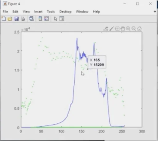
- The green dots show the result of the equalization without using the original value
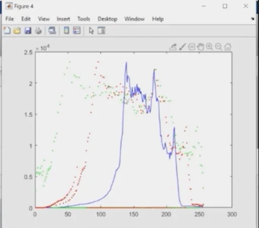
- The red dots show the result of the equalization using the original value
Caution
Gamma adjustment would not be great in this case, cuz we need to stretch the image out