Hybrid Images
Introduction
- Two different interpretations of a picture can be perceived by
- changing the viewing distance
- changing the presentation time
Generation of Hybrid Images
- generated by superimposing two images at two different spatial scales
Low-spatial Frequencies- Frequency cut of the low resolution
- The one that can be seen at a far distance
- An image that is filtered by low-pass filter
- Gaussian Filter
High-spatial Frequencies- Frequency cut of the high resolution
- The one that can be seen up close
- An image that is filtered by high-pass filter
- Laplacian Filter
The Perception of Hybrid Images
Note
Human observers can comprehend the meaning of a novel image within a short glance (100 msec)
- When observation time is limited, low frequencies are observed.
- Different durations lead to different results of observations.
Successful Hybrid Image
- When one percept dominates, it’s impossible to conciously switch between the alternative.
- Alternative can only be seen by the change of distance
- The
alternativemust be treated asnoises
1. What Does in Your Function
-
sigma_low→ controls how much of im1 is blurred. -
Small : keeps more detail (not blurry enough).
-
Large : very blurred, only coarse structure remains.
-
sigma_high→ controls how much of im2’s detail is kept. -
Small : subtracts only very fine details → result may look faint.
-
Large : subtracts a lot of content → result may contain too much, overpowering the hybrid.
So the balance is:
- Low-pass must preserve shape / identity of im1.
- High-pass must keep edges / texture of im2.
2. Use the Plotting Method to Guide Choice
Here’s how you can plot the frequency responses of your chosen sigmas and see if they complement each other well:
import numpy as np
import matplotlib.pyplot as plt

def plot_filters(sigma_low, sigma_high, fmax=60):
 f = np.linspace(0, fmax, 500)

 # Low-pass response
 H_low = np.exp(-(f**2) / (2 * sigma_low**2))

 # High-pass response
 H_high = 1 - np.exp(-(f**2) / (2 * sigma_high**2))

 plt.figure(figsize=(10,4))
 plt.plot(f, H_low, 'r', linewidth=2, label=f"Low-pass σ={sigma_low}")
 plt.plot(f, H_high, 'g', linewidth=2, label=f"High-pass σ={sigma_high}")
 plt.xlabel("Frequency (cycles/image)")
 plt.ylabel("Gain")
 plt.legend()
 plt.grid(True, linestyle=":")
 plt.title("Filter Frequency Responses")
 plt.show()

# Example:
plot_filters(sigma_low=8, sigma_high=20)- If the curves cross smoothly around 0.5 gain → you get something like fig (a) in your reference image.
- If there is a gap (both near 0 in mid frequencies) → you get something like fig (b). This means some frequencies are lost, making the hybrid less convincing.
3. Practical Way to Tune Sigmas
- Start with rule of thumb:
sigma_low≈ 8–12 (to blur im1 enough to remove detail but keep recognizability).sigma_high≈ 2–6 (to extract edges from im2).
- Plot the filter curves with the function above.
- Make sure the low-pass is strong at low frequencies and has faded out before the high-pass kicks in.
- Check the hybrid in Fourier domain:
- Plot radial spectrum of your hybrid and overlay filters.
- You’ll see whether your chosen sigmas complement each other (no big gap, no big overlap).
4. What to Look For in a “Good” Hybrid
- Near range (look close): High frequencies dominate → you should see im2.
- Far range (look far or zoom out): High frequencies disappear → you should see im1.
That only happens if your frequency split is clean — which is why plotting the curves is so useful.
Rules of Perceptual Grouping and Hybrid Image
1. Fewer elements in low spatial frequncies
- Low spatial frequencies (blob)
lackaprecise definitionof object shapes andregion boundaries - Users tend to interpret elements in the simplest way possible.
2. Avoid symmetry and repetitiveness in low spatial frequencies
- Symmetry and repetitiveness forms a strong percept that is hard to eliminate perpetually.
- The patterns would always remain visible even when viewing from a short distance
3. Color provides a very strong grouping cue
- Color is used only in the high frequencies
4. Choosing a proper cut-off frequencies for the filter
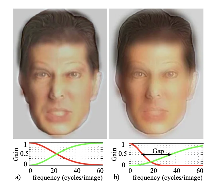
- Avoid strong filter overlap to provide unambiguous interpretation when viewing from different distances away.
Correlation and Hybrid Image
Important
Scale, Edge, and Frequencies
- Scale: The level of detail or resolution
- coarse scale: low frequencies, blurs away details
- fine scale: high frequencies, preserves details
- Edge
- where the sharp changes occurs in intensity or color
- local minima in the image gradient
- Frequencies
- How rapidly intensity changes over a short distance
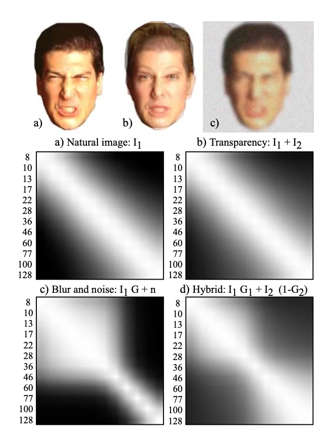
a)
- The edges found at one scale are correlated with the edges found in the scales below and above.
b)
- The same when two images are superimposed (additive transparency).
c)
- The same also holds when an image is blurred.
d)
- The correlation is corrupted when white noises are added.
Subband and Scale
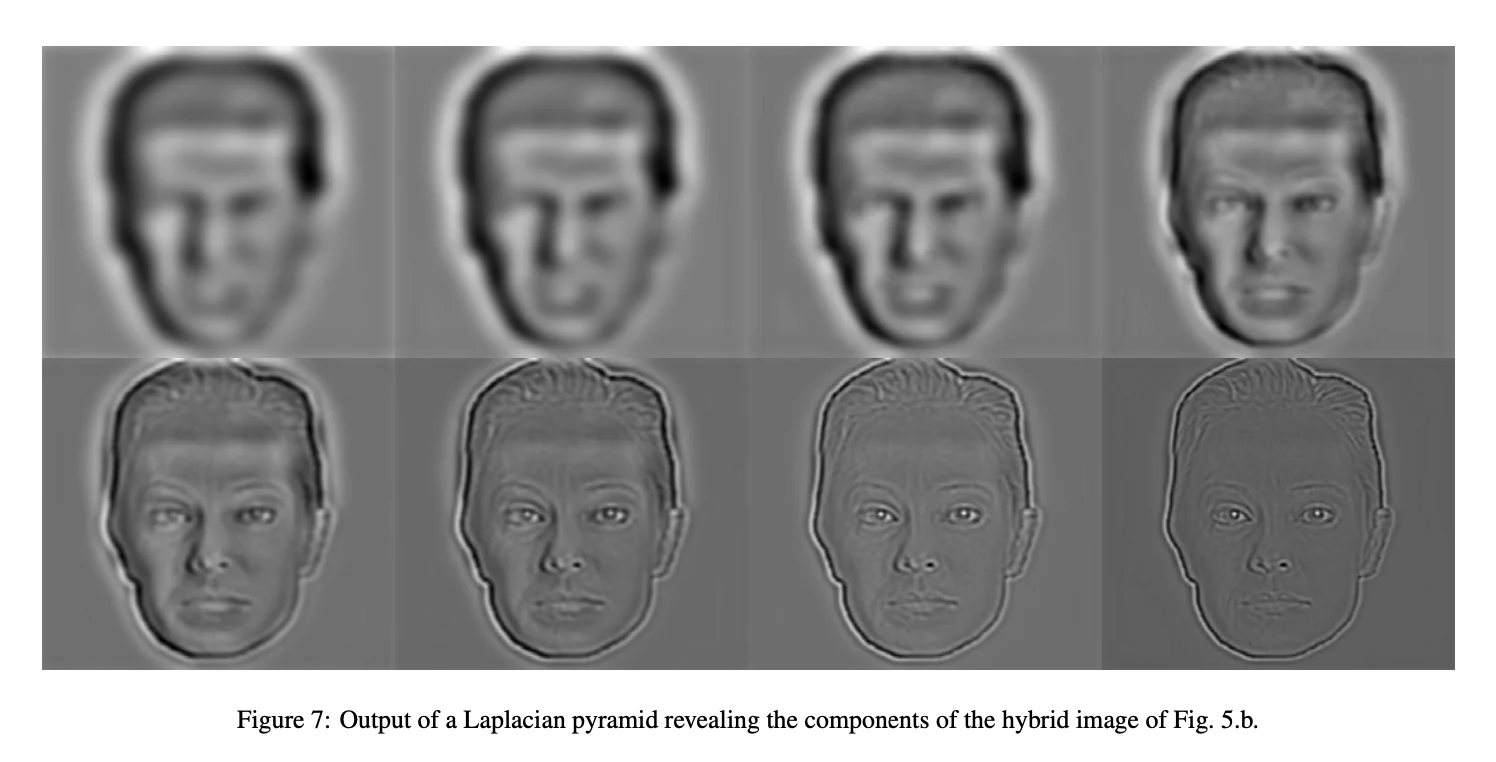
Note
- High frequencies: a stern woman
- Low frequencies: an angry man
- Each subband is also a hybrid image.
- The finer the scale of each subban, the farther you have to go in order to see the switch of images