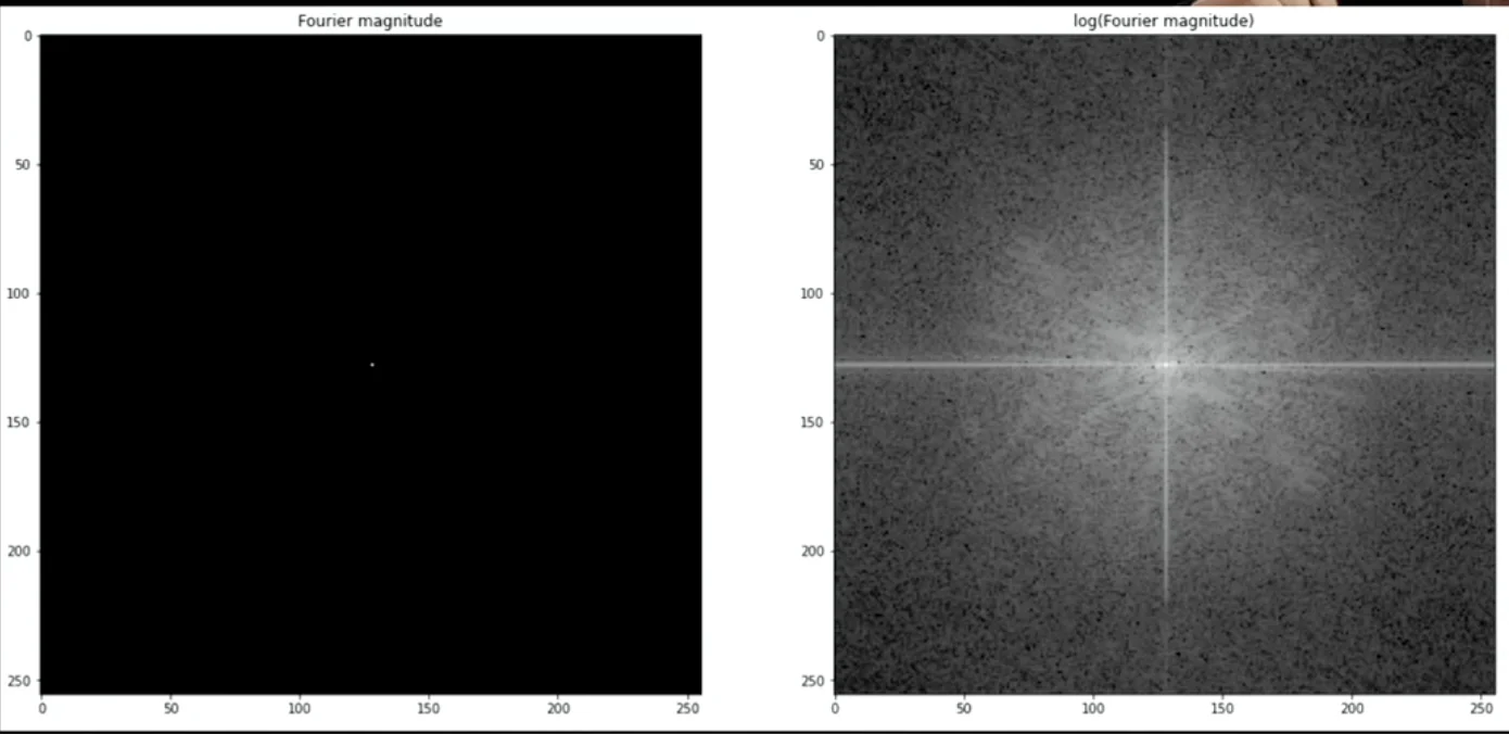
Magnitude and Its Log-form of the Fourier Transform
import numpy as np
import matplotlib.pyplot as plt
from numpy import fft
f = plt.imread("al.jpg")
F = fft.fftshift(
fft.fft2(f))
Fmag = np.abs(F)# Plotting
fig,(ax1, ax2)= plt.subplots(1,2, figsize=(20,10))
ax1.set_title("Fourier Magnitude")
ax1.imshow(Fmag, cmap="gray")
ax2.set_title("Log Fourier Magnitude")
ax2.imshow(np.log(Fmag), cmap="gray")
fft.fftshift: shift the origin of the coordinate system from the top-left corner to the center
fft.fft2(f): calculate the fourier transform of the image
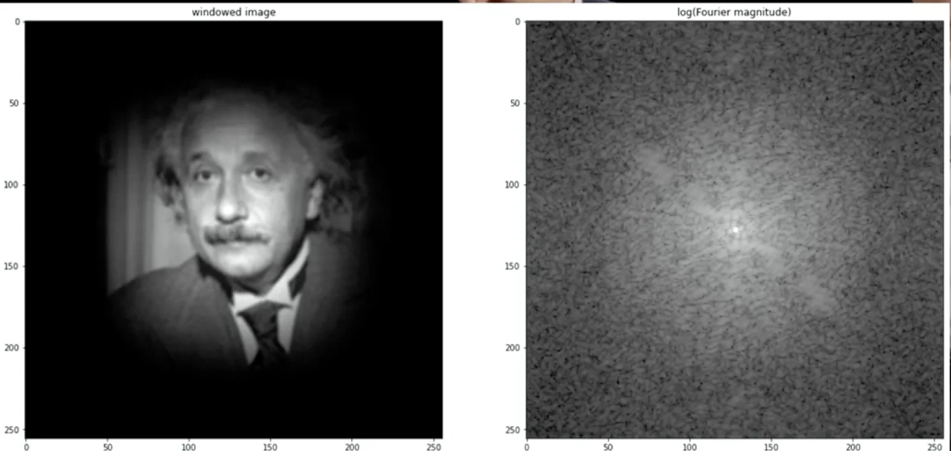
In the center of the image, there is a DCTerm representing the average pixel intensity of the entire image.
The DCTerm is so strong that the other values are comparatively small and nearly invisible
The np.log(Fmag) resolves this problem
Creating a window smoothly tapers to zero at all four edges
f = plt.imread(al.jpg)[ydim, xdim]= f.shape
win = np.outer(
np.hanning(ydim),
np.hanning(xdim),)
win = win / np.mean(win)# make unit-mean
F = fft.fftshift(fft.fft2(f * win))
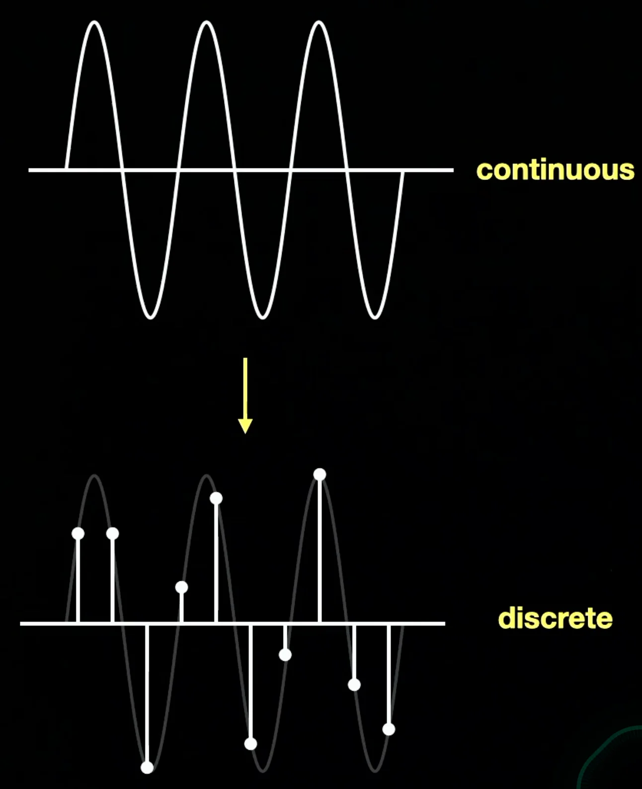
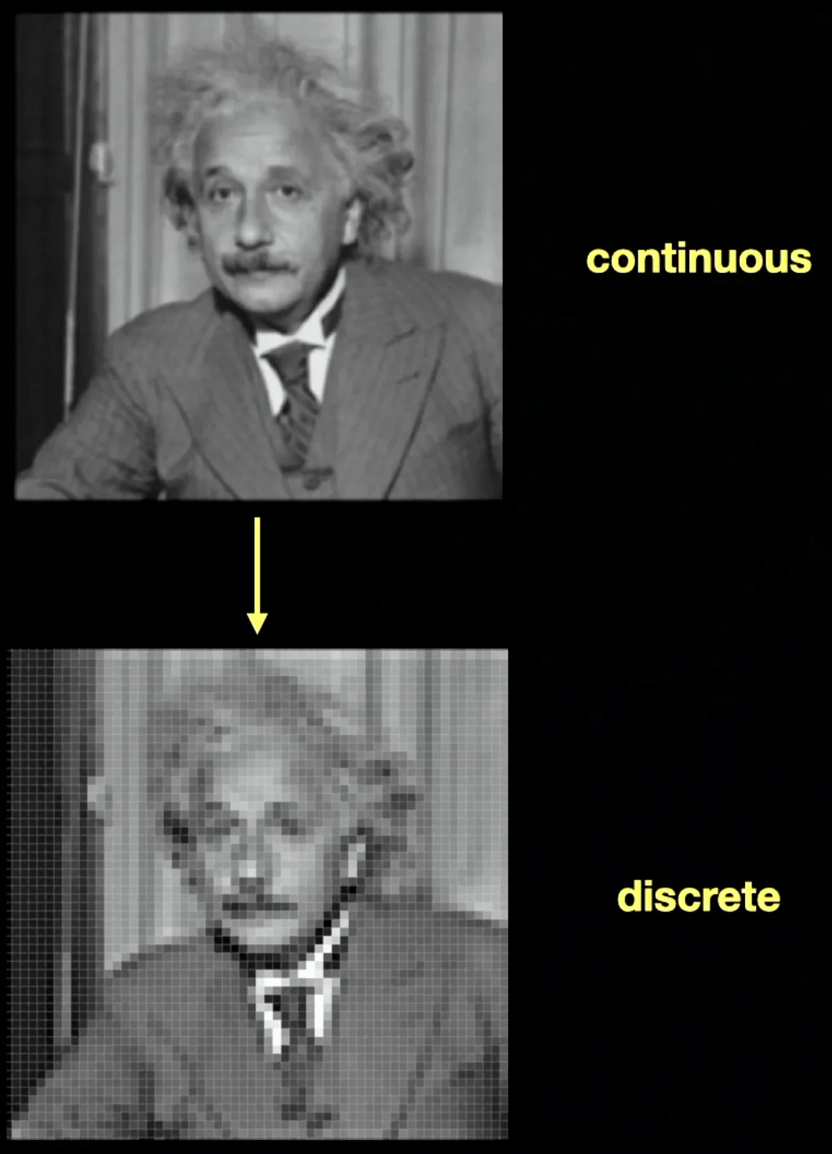
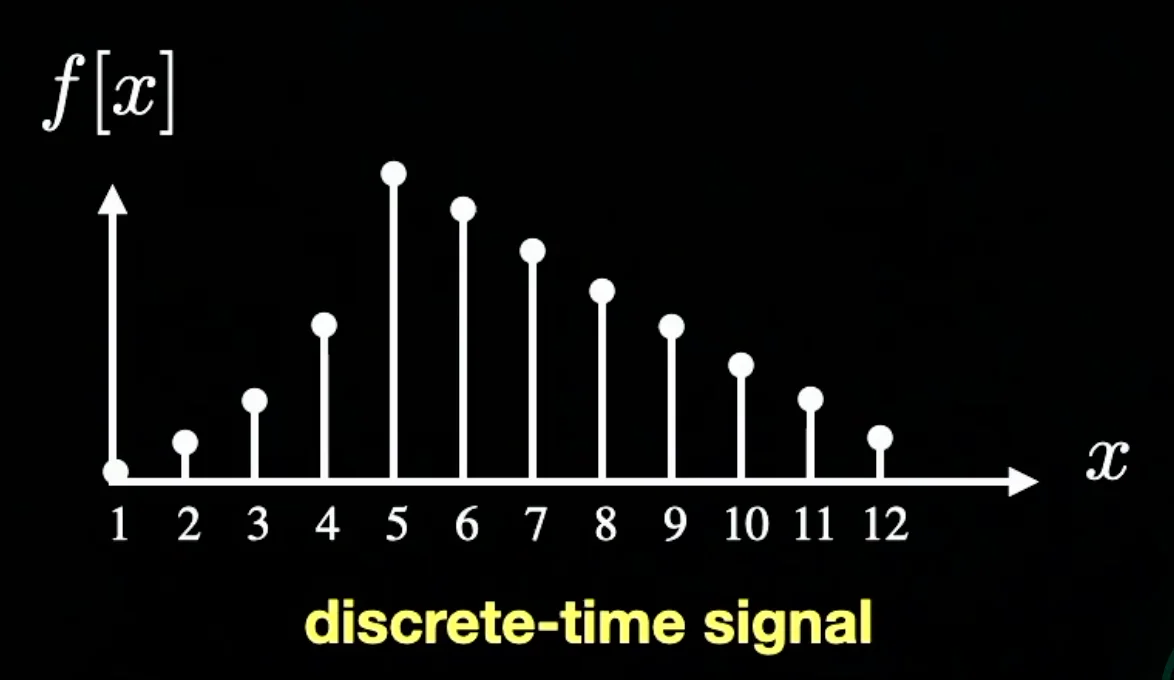
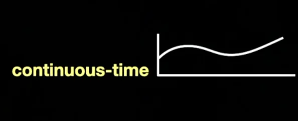
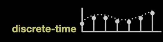
Continuous to Discrete Sampling
f(x)
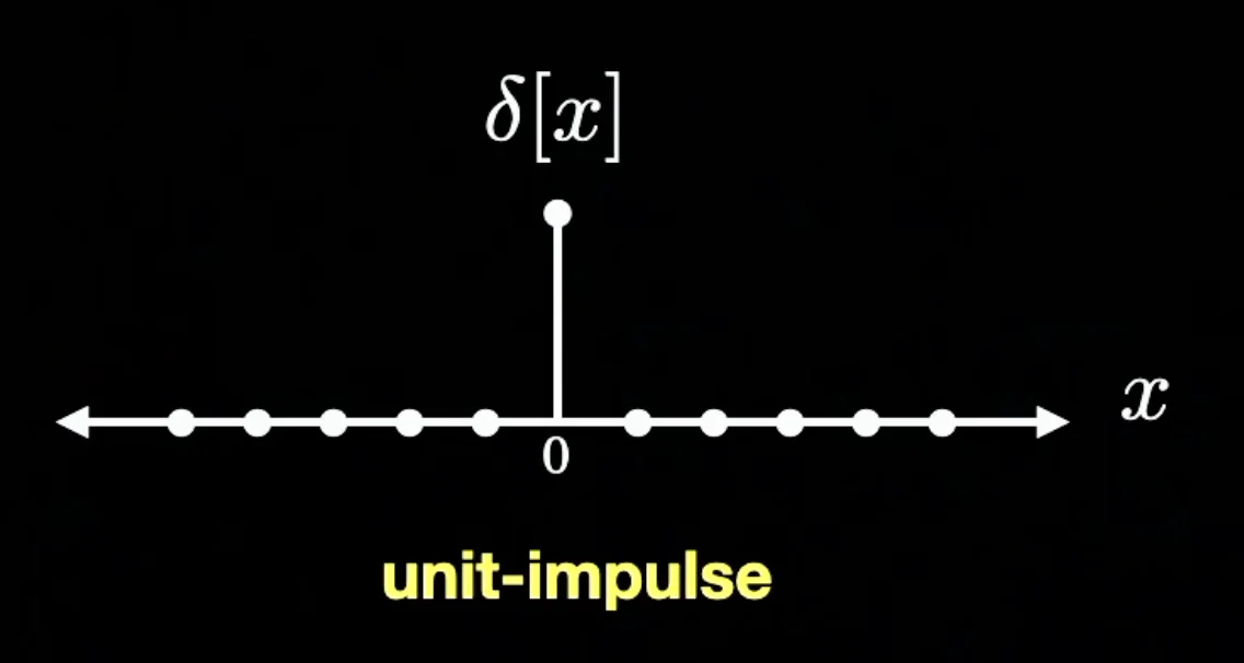
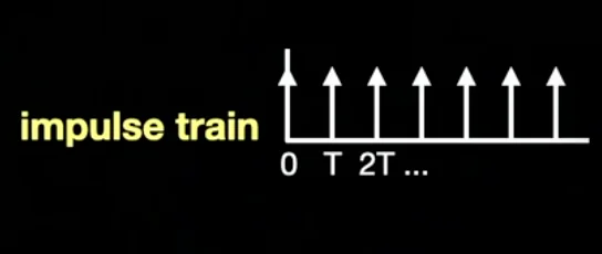
s(x)=∑k=−∞∞δ(x−kT)
Sampling
T: How fine we want to sample
Tip
δ(x)={1(x=0)0(x=0)
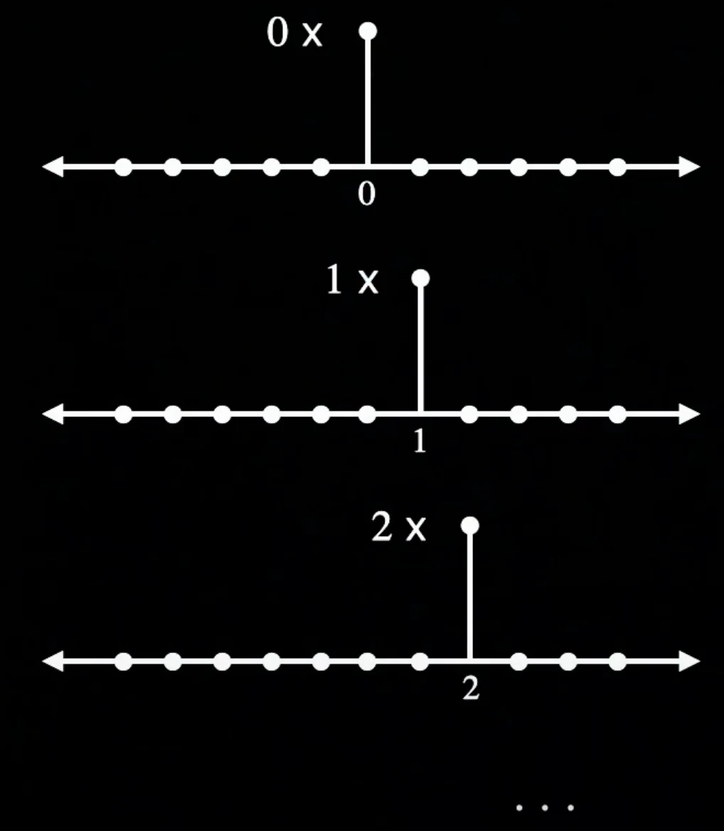
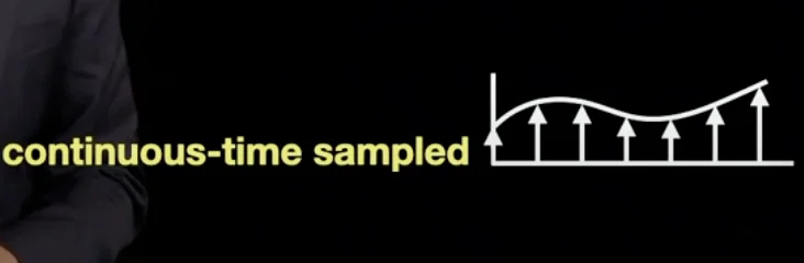
fs(x)=f(x)s(x)
grabbing the values that we want but having 0 everywhere else
f[x]=fs(xT)
Take each integer multiples of T
Convolution and Fourier Transform
Formulas
fs(x)=f(x)s(x)⇒Fs(x)=F(ω)∗S(ω)
Important
The convolution in the frequency domain is the same as the multiplication in the spatial domain, and vice versa.
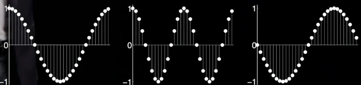
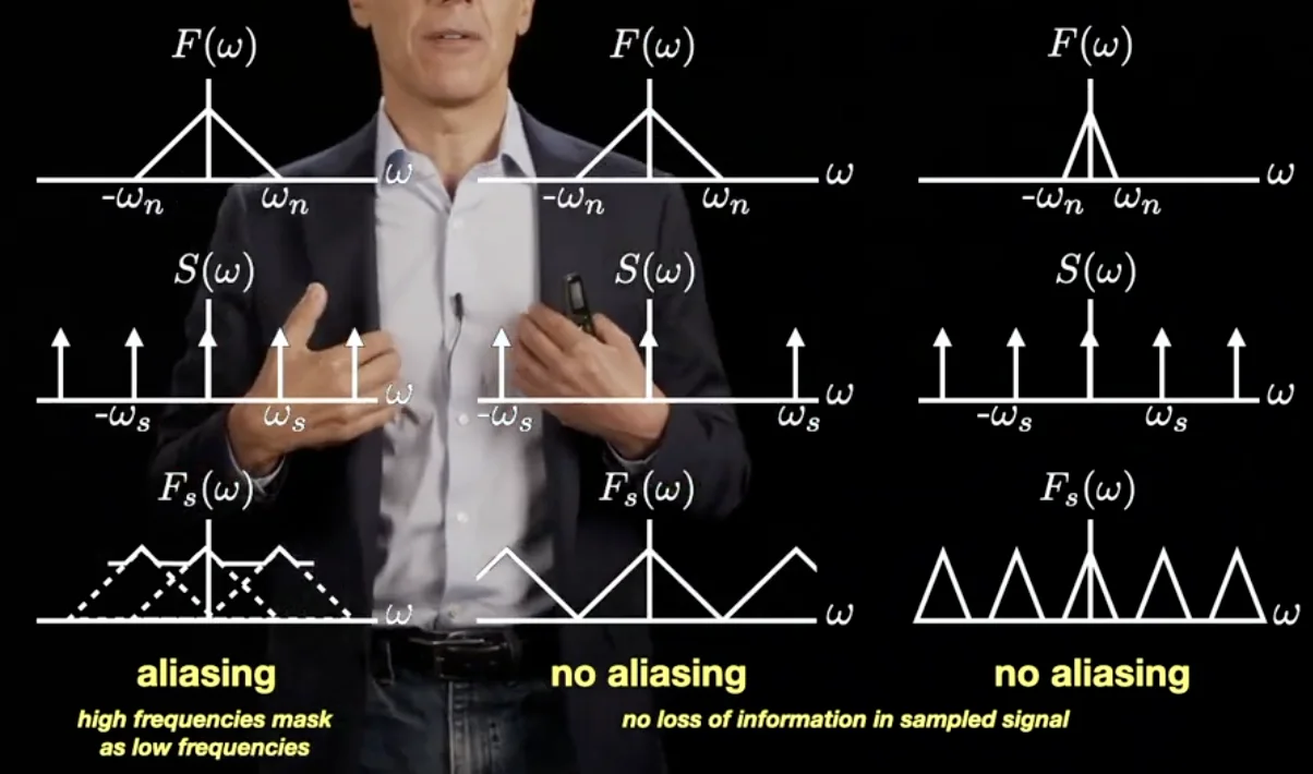
What do we lose when we samples
∙ Aliasing
Aliasing causes artifacts and the loss of information in the image
∙ Nyquist Limit
ωs>2ωn
A solution to determining aliasing
Perfect representation of a signal without information loss
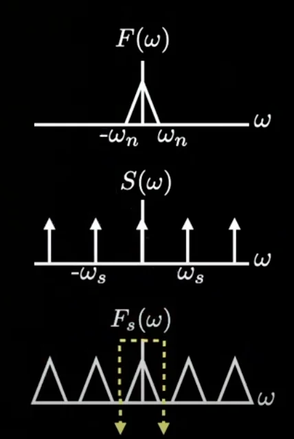
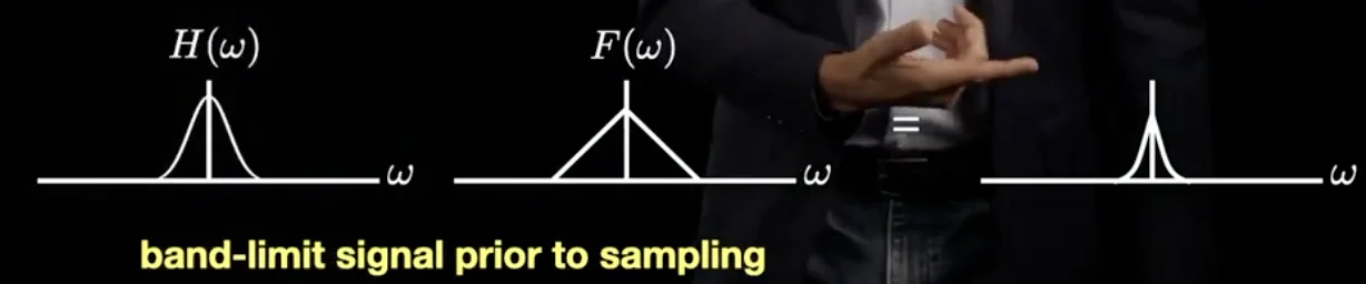
Prevent Replicates
Sampling induces replicate signals
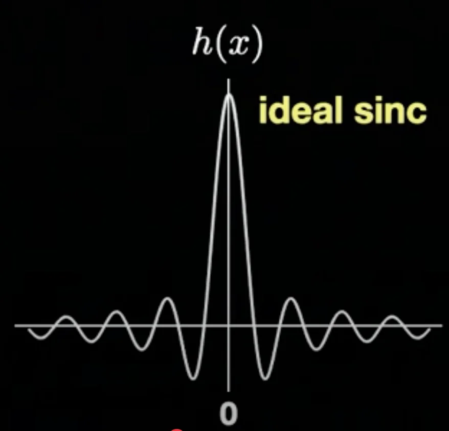
Apply ideal sinc to resolve this problem
h(x)=Tπxsin(Tπx)
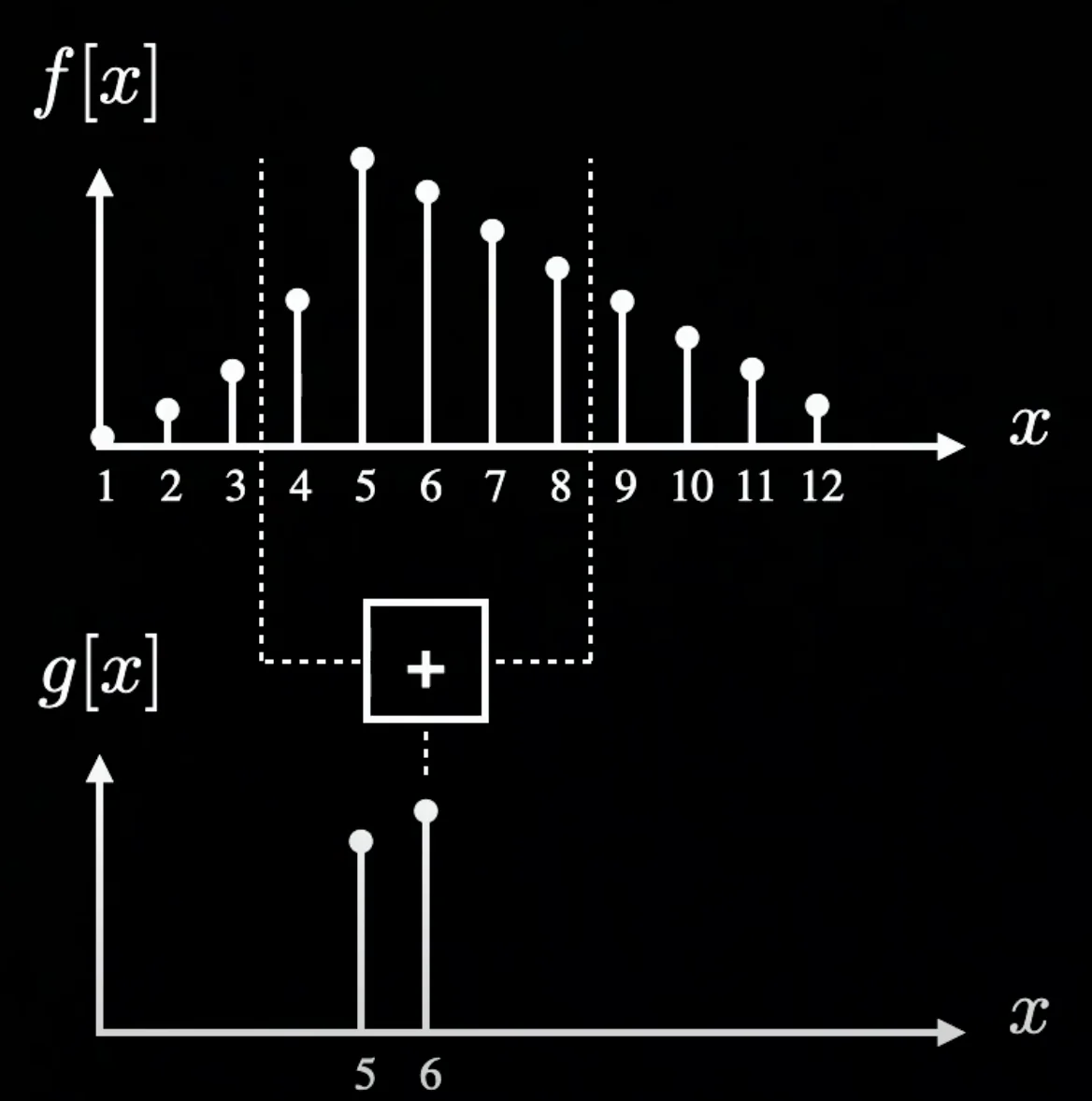
Discrete to Discrete Sampling
Discard high frequency part of the image and down-sample it
Given Gaussian Function h(x)=e−x2/σ2
Spatial Domain
g[x]=(h(x)∗f[x])s[x]
Frequency Domain
G[ω]=(H(ω)F[ω])∗S[ω]
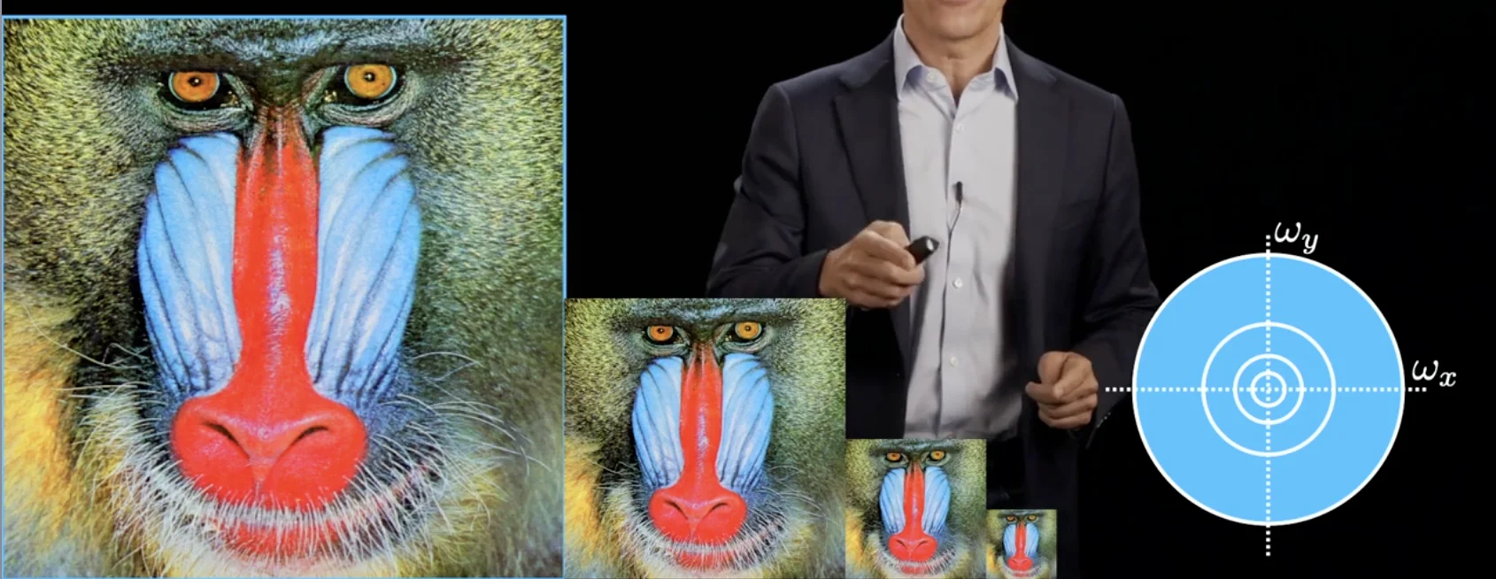
The signal becomes narrower, which means the higher frequencies are filtered successfully
Aliasing would not happen
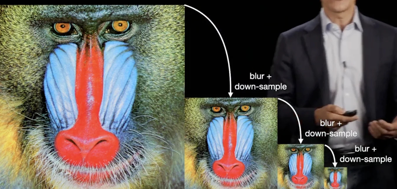
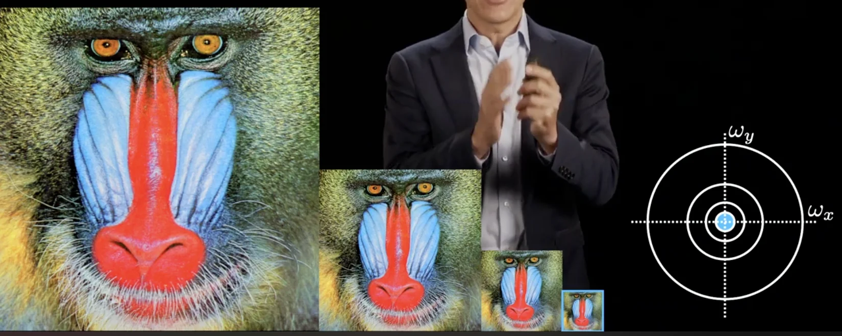
Gaussian Pyramid
Repeated process of blurring + down-sampling
blurring is typically done with Gaussian Filter
In Fourier Domain
Code
im = plt.imread("mandrill.png")# load image
h =[1/16,4/16,6/16,4/16,1/16]# unit-sum blur filter (a Gaussian filter)
N =3# pyramid level
P =[im]for k inrange(1, N):
im2 = np.zeros(im.shape)for z inrange(3):
im2[:,:, z]= sepfir2d(im[:,:, z], h, h)# blur each color channel
im2 = im2[0:-1:2,0:-1:2,:]# down-sample by 2 x 2
im = im2
P.append(im2)
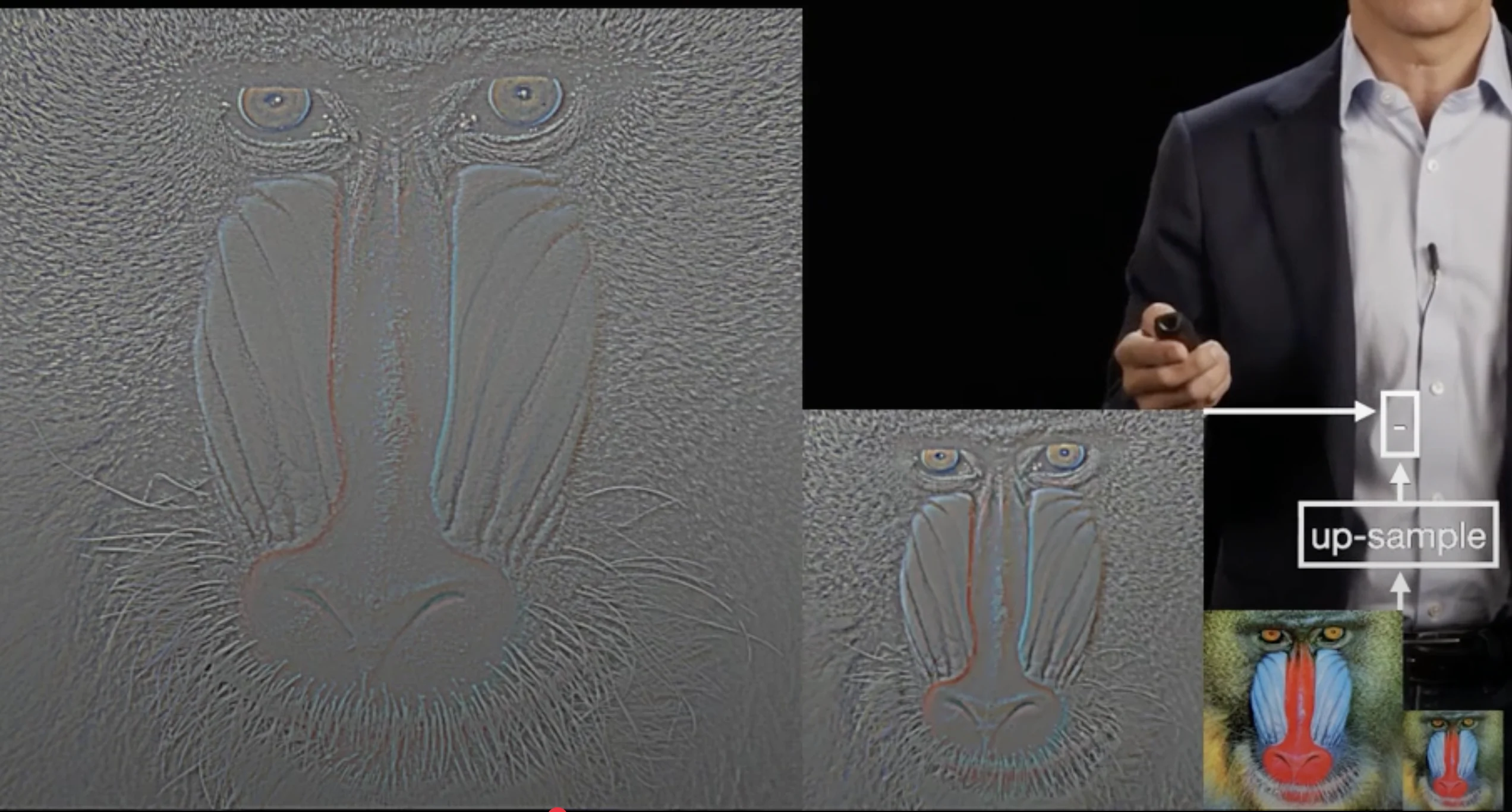
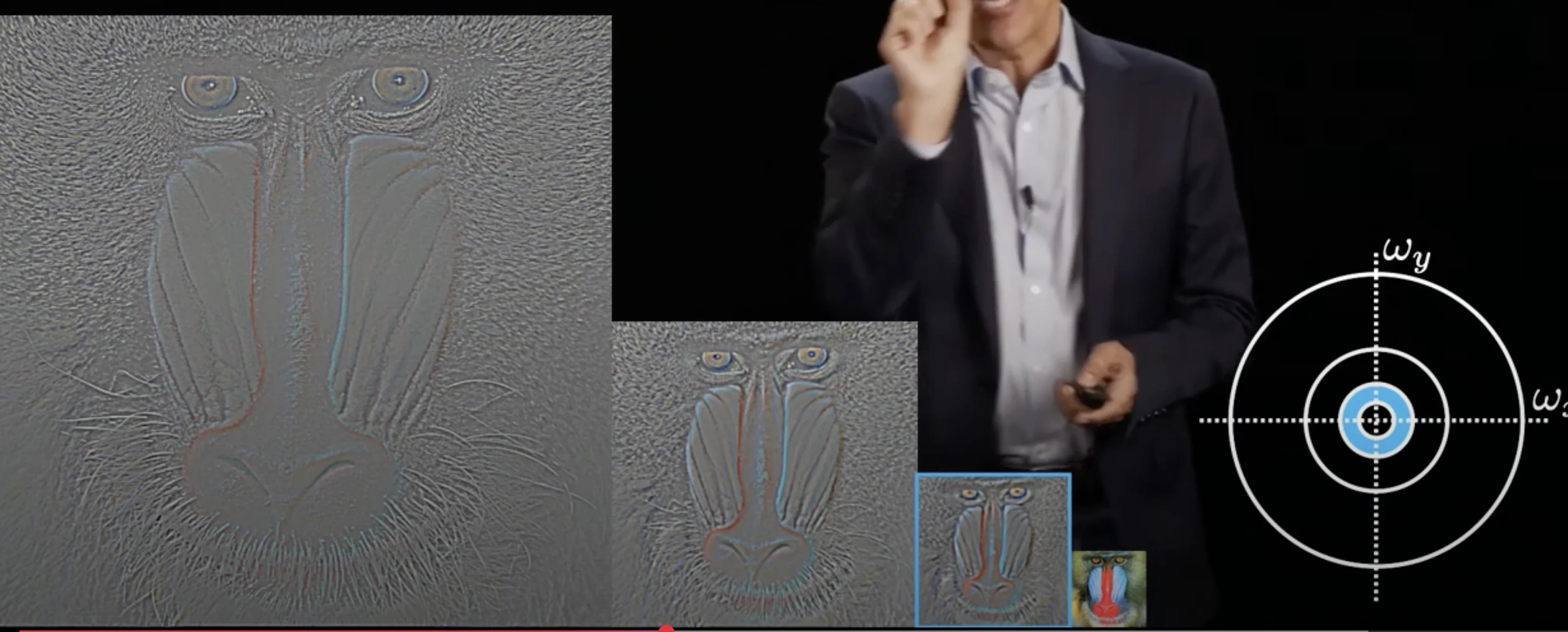
Laplacian Pyramid
Starting from a Gaussian Pyramid
Repeated of up-sampling and subtraction
In Fourier Domain
Code
L =[]for k inrange(0, N -1):
l1 = G[k]
l2 = G[k +1]
l2 = cv2.resize(l2,(0,0), fx=2, fy=2)# up-sample
D = l1 - l2
D = D - np.min(D)# scale in [0, 1]
D = D / np.max(D)# for display purpose
L.append(D)
L.append(G[N -1])