1-1. Nonparametric Methods
Introduction
Parametric methods
- use of probability distributions that have specific functional forms governed by a small number of parameters whose values are to be determinied from a data set.
Caution
LIMITATION
- The chosen density might be a poor model of the distribution that generates the data resulting in poor predictive performance
- Gaussian distribution cannot capture multimodal data
Nonparametric Methods
- Consider a case of a single continuous variable .
- Using a standard historgrams to partition into distinct bins:
- : index of bin
- : width of bins
- : the number of falling in bin
Normalized Probability Density
- The bins to obtain probability values:
- Where:
Example - Histogram
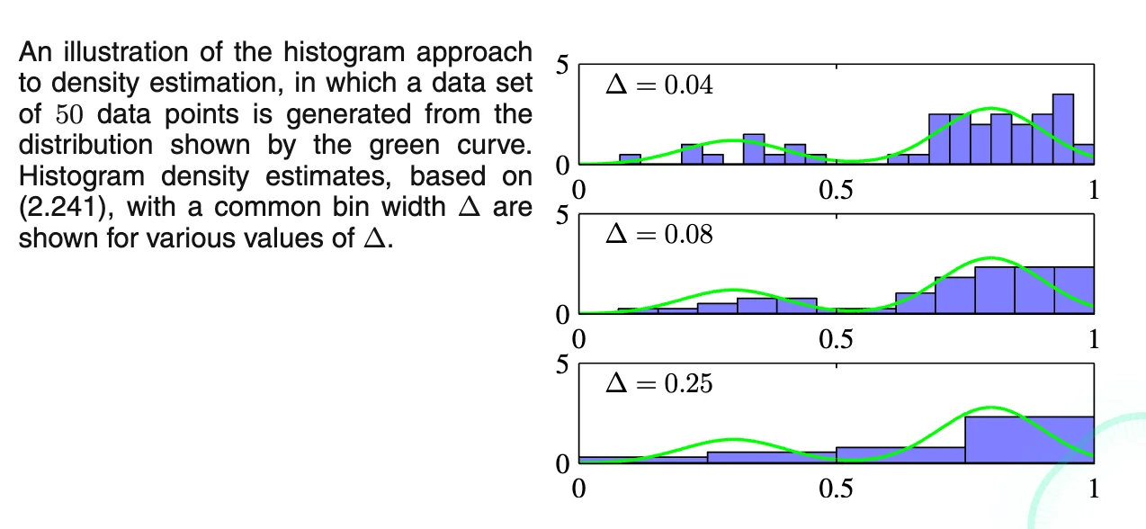
- Data is formed from a mixture of
2 Gaussians - small
- with a lot of structure that is not present in the underlying distribution
- large
- fails to capture the bimodal property
Tip
ADVANTAGES
- Data set can be discarded after histogram is generated
- Easily applicable if data points arrive sequentially
Caution
LIMITATION
- Discontinuities occur due to bin edges rather than the properties of underlying distributions
- When data are in a high-dimensional space, we would experience
Takeaway from Histogram
- Consider the points lie in local neighborhoods (the bins in histogram)
- Some distance measurements are required
- Smoothing parameter should be neither too large nor too small.
Kernel Estimator
- Assume observations are drawn from a probability density in D-dimensional space.
- Consider a small region containing
The probability associated with the region
The probability distribution of the total number of K points falling within the region
For large N, the peak is around the mean of K
Important
Mean of (the count)
Mean of (the fraction)
If is sufficiently small
- where is the volume of
Combine and
Different Exploitations of
Fix K, determine V
- KNN density estimator
Fix V, determine K
- Kernel Approach
Note
Both converge to the true probability density in the limit with shrinking with , and growing with
Kernel Method
-
Take the region to be a small hypercube centered on the point
-
is the point where we wanna determine the probability density.
- helps to count the # of points falling within
- represents a unit cube centered on the origin
- is a kernel function called
Parzen Window
-
if in a cube of side centered on x, and 0 otherwise
-
Total # of the datapoints in cube
- Swap the total into probability density with
- To prevent artificial discontinuities, we can user smoother kernel functions (i.e. Gaussian)
- is the standard deviation
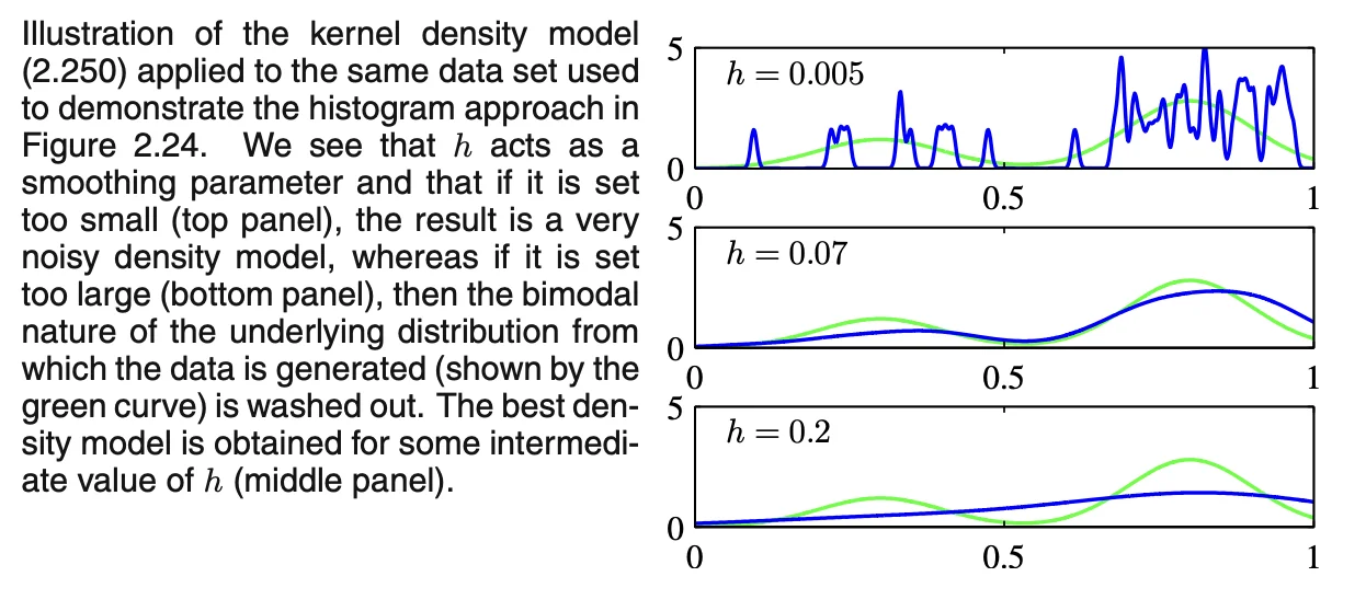
Tip
- Any kernel methods satisfying the following conditions can be chosen.
- No computational cost during the training time
Caution
Kernel approach may lead to over-smoothing due to that the parameter governing the kernel width is fixed for all kernels
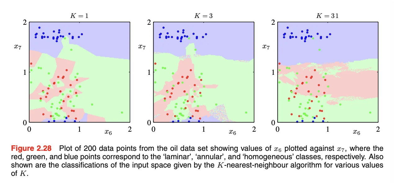
KNN Methods
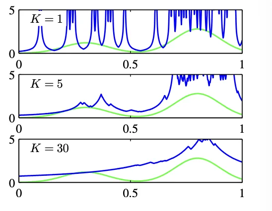
- The parameter governs the degree of smoothing.
Method
- Assume a data set of sizes with points in class
- Draw a
spherecentered on a new point containing points - : Volume of the
sphere - : points from class
- The estimate of the density associated with each class
- Unconditional Density
- Priors
- Posteriors
Note
In the case where K = 1, the KNN is called “the nearest-neighbor” approach