1-2 Intro to ML Concepts
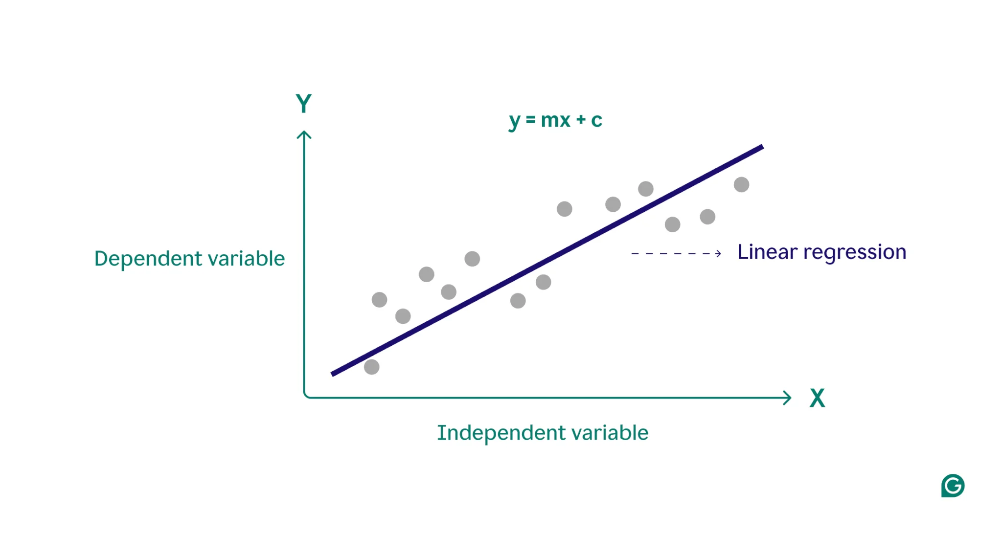
Linear Regression
- Inductive Bias
- Assumtptions about the nature of the data distribution
- p(y∣x) for
supervised problem
- p(x) for
unsupervised problem
- Parametric Model
- A statistical model with a fixed number of parameters
∙ Formula for Linear Regression
y(x)=w⊺x+ϵ
- ϵ
- Residual error between our lienar prediction and the true responses
- ∼N(μ,σ2)
∙ Linear Regression and Gaussian
p(u∣x,θ)=N(y∣μ(x),σ2(x))
- μ is a linear function of x s.t. μ=w⊺x
- For 1-D data:
- μ(x)=w0+w1x=w⊺x
- σ2(x) is the noise fixed: σ2(x)=σ2
∙ Estimation via Residual Sum of Squares
- Objective: minimize the sum of squared residuals
RSS(w)=i=1∑n(yi−w⊤xi)2
w∗=argwminRSS(w)
l:y=ax+b(prediction)L=i=1∑n(yi−axi−b)2(RSS)
∂a∂L=0∂b∂L=0
∂a∂=i=1∑n(yi−axi−b)2=i=1∑n2(yi−axi−b)(−xi)=2i=1∑n(−xiyi+axi2+bxi)∵∂L∂a=0∴i=1∑n(−xiyi+axi2+bxi)=0⇒−n(σxy−y^x^)+an(σx2+x^2)+bnx^=0⇒−(σxy+y^x^)+a(σx2+x^2)+bx^=0
∂b∂=i=1∑n(yi−axi−b)2=i=1∑n−2(yi−axi−b)=−2i=1∑n(yi−axi−b)∵∂L∂b=0∴i=1∑n(yi−axi−b)=0⇒−ny^+anx^+bn=0⇒−y^+ax^+b=0
{a(σx2+x^2)+bx^−(σxy+y^x^)=0ax^+b−y^=0⇒b=y^−ax^⇒aσx2+ax^2+y^x^−ax^2−σxy−y^x^=0⇒a=σx2σxy(regression coefficient)⇒b=y^−σx2σxyx^
∵a=σx2σxyb=y^−σx2σxyx^∴y=ax+b⇒y=σx2σxyx+y^−σx2σxyx^⇒y−y^=σx2σxy(x−x^)⇒y−y^=σxσyσxy⋅σxσy(x−x^)⇒y−y^=ρxy⋅σxσy(x−x^)
- Closed-form solution (Normal Equation):
w∗=(X⊤X)−1X⊤y
where X is the design matrix.
Note
DESIGN MATRIX
X=11⋮1x11x21⋮xn1x12x22⋮xn2⋯⋯⋱⋯x1dx2d⋮xnd
- Rows correspond to observations (data points).
- Columns correspond to features (including the constant 1 for intercept).
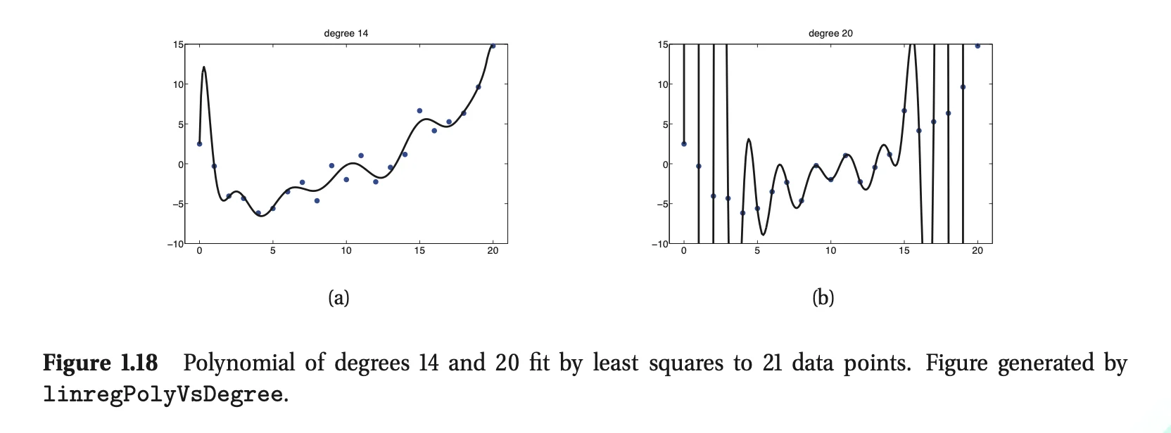
∙ Linear regression with non-linear relationships
- Polynomial Regression
- Replace x with some non-linear functions
p(u∣x,θ)=N(y∣w⊺ϕ(x),σ2)
- Basis function expansion
- e.g. ϕ(x)=[1,x,x2,…,xd], for d=14 and d=20
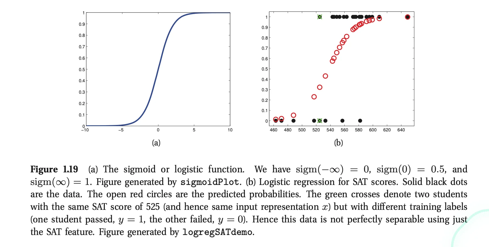
Logistic Regression
- Generalize Linear Regression to the binary classification
1. Replace Gaussian Distribution to Bernoulli Distribution
p(y∣x,w)=Ber(y∣μ(x))
- y∈{−1,1}
- μ(x)=E[y∣x]=p(y=1∣x)
2. Pass μ(x) through sigmoid function
sigm(η)≜1+e−η1=eη+1eη
μ(x)=sigm(w⊺x)
- The squashing function sigmoid maps the whole real line to [0,1]
p(x∣x,w)=Ber(y∣sigm(w⊺x))
3. Example: p(yi=1∣xi,w)=sigm(w0+w1xi)
Model Selection
- We can decide on which model to select based on the
misclassification rate
err(f,D)=N1i=1∑NI(f(xi)=yi)⋅where I(f(xi)=yi)={1(f(xi)=yi)0(f(xi)=yi)
- Example of an increased error rate due to the increase in K. (
over-smoothing)
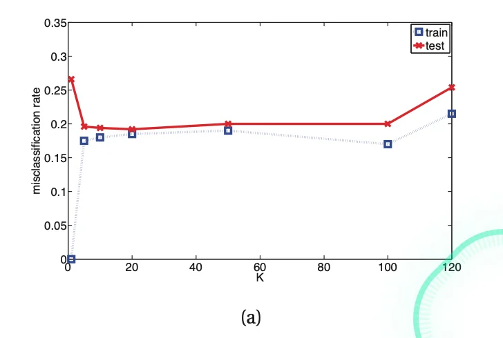
- For complex models (small K), the method
overfits
- For simple models (large K), the method
underfits
Validation
- Create a test set by partitioning data into different parts
- usually 80% for training and 20% for testing
∙ Cross Validation
- Split data into K folds. For each fold k∈{1,…,K}, we train on all data but the kth fold.
- We test our trained model on the kth fold.
- Leave-one out cross validation (LOOCV)
- set K=N, leaving 1 test case for validation