2. Perceptron
Linear Separability
A set of examples is linearly separable if there exists a linear decision boundary that can separate the points
Perceptron
Perceptron is a linear classifier that only converges when data is linearly separable .Dataset: D = { x ( i ) , y ( i ) } N i D = \{{x^{(i)}, y^{(i)}}\}^{i}_{N} D = { x ( i ) , y ( i ) } N i Assumptions: Binary classification: y ∈ { − 1 , + 1 } y \in \{-1, +1\} y ∈ { − 1 , + 1 }
Data is linearly separable
The only hyperparameter in the perceptron is the max number of iterations
Too many iterations may lead to overfit
Too few iterations may lead to underfit
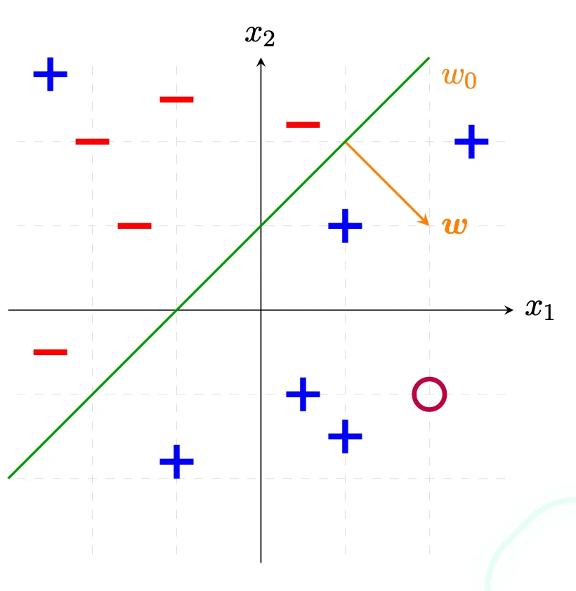
Hyperplane
H = { x : w ⊺ x + w 0 = 0 } ⇒ w ⋅ x = 0 \begin{align*}
H &= \{x: w^\intercal x + w_0 = 0\} \\
&\Rightarrow w \cdot x = 0
\end{align*} H = { x : w ⊺ x + w 0 = 0 } ⇒ w ⋅ x = 0
The bias term w 0 w_0 w 0 threshold that allows the activation value to be increased by some fixed value b.
Positive Example
w ⊺ x + w 0 > 0 w^\intercal x + w_0 > 0 w ⊺ x + w 0 > 0 Negative Example
w ⊺ x + w 0 < 0 w^\intercal x + w_0 < 0 w ⊺ x + w 0 < 0 Classifier
h ( x ) = s i g n ( w ⊺ x + w 0 ) h(x) = sign(w^\intercal x + w_0) h ( x ) = s i g n ( w ⊺ x + w 0 ) Updating w
What the perceptron does.
w ← w + y ( i ) x ( i ) w \leftarrow w + y^{(i)}x^{(i)} w ← w + y ( i ) x ( i )
Why is w w w
w ⋅ x = 0 w \cdot x = 0 w ⋅ x = 0 x x x As w ⋅ x = 0 w \cdot x = 0 w ⋅ x = 0 w w w
Example
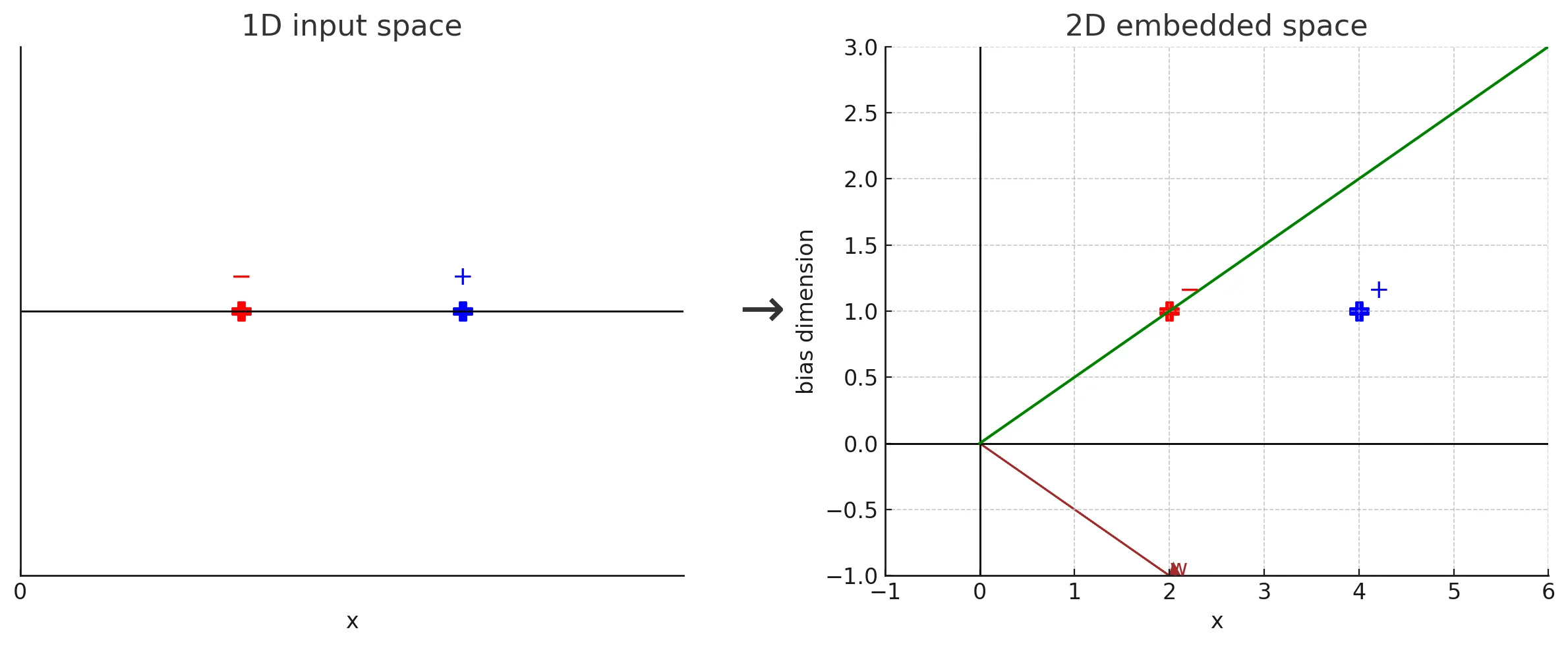
Notational Hack
w ⊺ x + w 0 ⇒ w ⊺ x w^\intercal x + w_0 \Rightarrow w^\intercal x w ⊺ x + w 0 ⇒ w ⊺ x
As we rewrite the notations as follows:
x =
\begin{bmatrix}
x_1 \
\vdots \
x_d
\end{bmatrix}
\Rightarrow
\begin{bmatrix}
\uparrow \
x \
\downarrow \
1
\end{bmatrix}
2. $$
w =
\begin{bmatrix}
w_1 \\
\vdots \\
w_d
\end{bmatrix}
\Rightarrow
\begin{bmatrix}
\uparrow \\
w \\
\downarrow \\
w_0
\end{bmatrix}
The result of this rewrite (increment dimensionality by 1)
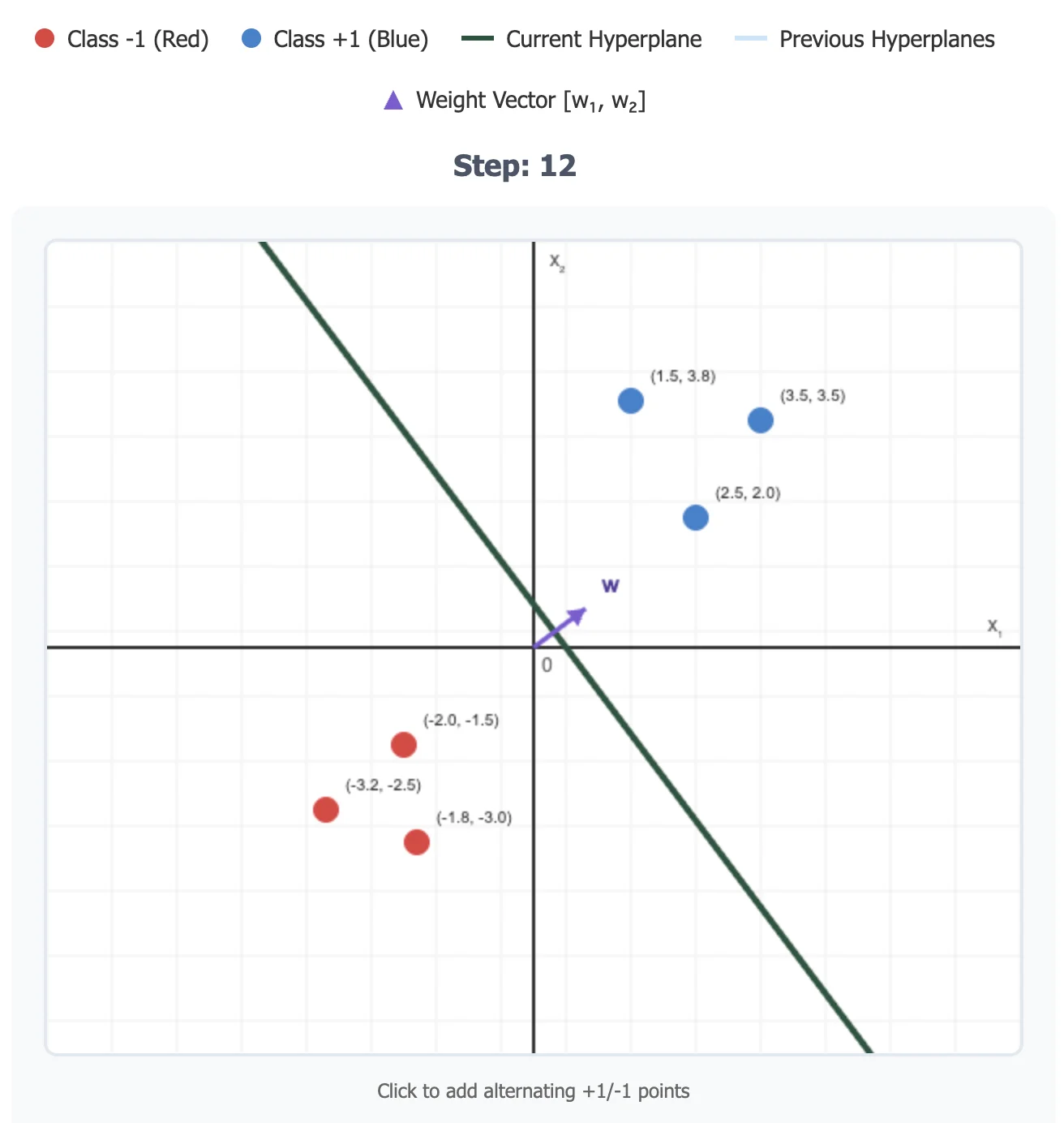
Perceptron Algorithm
Algorithm
PerceptronTrain ( D , M a x I t e r ) 1 : w d ← 0 , for all d = 1 … D // initialize weights 2 : b ← 0 // initialize bias 3 : for i t e r = 1 … M a x I t e r do 4 : for all ( x , y ) ∈ D do 5 : a ← ∑ d = 1 D w d x d + b // compute activation for this example 6 : if y a ≤ 0 then 7 : w d ← w d + y x d , for all d = 1 … D // update weights 8 : b ← b + y // update bias 9 : end if 10 : end for 11 : end for 12 : return w 0 , w 1 , … , w D , b \begin{array}{l}
\hline
{\text{PerceptronTrain}}(D, MaxIter) \\
\hline
\begin{array}{ll}
1: & w_d \leftarrow 0, \text{ for all } d = 1 \ldots D & \text{// initialize weights} \\
2: & b \leftarrow 0 & \text{// initialize bias} \\
3: & \textbf{for } iter = 1 \ldots MaxIter \textbf{ do} \\
4: & \quad \textbf{for all } (x,y) \in D \textbf{ do} \\
5: & \quad \quad a \leftarrow \sum_{d=1}^D w_d x_d + b & \text{// compute activation for this example} \\
6: & \quad \quad \textbf{if } ya \leq 0 \textbf{ then} \\
7: & \quad \quad \quad w_d \leftarrow w_d + y x_d, \text{ for all } d = 1 \ldots D & \text{// update weights} \\
8: & \quad \quad \quad b \leftarrow b + y & \text{// update bias} \\
9: & \quad \quad \textbf{end if} \\
10: & \quad \textbf{end for} \\
11: & \textbf{end for} \\
12: & \textbf{return } w_0, w_1, \ldots, w_D, b \\
\end{array} \\
\hline
\end{array} PerceptronTrain ( D , M a x I t er ) 1 : 2 : 3 : 4 : 5 : 6 : 7 : 8 : 9 : 10 : 11 : 12 : w d ← 0 , for all d = 1 … D b ← 0 for i t er = 1 … M a x I t er do for all ( x , y ) ∈ D do a ← ∑ d = 1 D w d x d + b if y a ≤ 0 then w d ← w d + y x d , for all d = 1 … D b ← b + y end if end for end for return w 0 , w 1 , … , w D , b // initialize weights // initialize bias // compute activation for this example // update weights // update bias Python
def perceptron ( D: DataSet, w: WeightVector) :
w = [ 0 , 0. . . 0 ] . T
while True :
changed = False
for i in range ( N) :
if y[ i] * ( w @ x[ i] ) <= 0 :
w = w + y[ i] * x[ i]
changed = True
if not changed:
break Why y ( i ) ( w ⊺ x ( i ) ) ≤ 0 y^{(i)}(w^\intercal x^{(i)}) \le 0 y ( i ) ( w ⊺ x ( i ) ) ≤ 0
y ∈ { 1 , − 1 } y \in \{1, -1\} y ∈ { 1 , − 1 }
Error-driven Updating: Only update the weights if a prediction is wrongIf the updated w w n e w w_{new} w n e w
y ( w n e w ⊺ x ) = y ( ( w + y x ) ⊺ x ) = y ( w ⊺ x + y x ⊺ x ) = y ( w ⊺ x ) + y y x ⊺ x = y ( w ⊺ x ) + ∣ ∣ x ∣ ∣ 2 > y ( w ⊺ x ) \begin{align*}
&y(w_{new}^\intercal x ) \\
&= y((w + yx)^\intercal x) \\
&= y(w^\intercal x + yx^\intercal x) \\
&= y(w^\intercal x) + yyx^\intercal x \\
&= y(w^\intercal x) + ||x||^2 \\
&> y(w^\intercal x)
\end{align*} y ( w n e w ⊺ x ) = y (( w + y x ) ⊺ x ) = y ( w ⊺ x + y x ⊺ x ) = y ( w ⊺ x ) + yy x ⊺ x = y ( w ⊺ x ) + ∣∣ x ∣ ∣ 2 > y ( w ⊺ x )
( w ⊺ x ( i ) ) (w^\intercal x^{(i)}) ( w ⊺ x ( i ) ) w ⋅ x ( i ) > 0 w\cdot x^{(i)}> 0 w ⋅ x ( i ) > 0 The input vector points to the same general direction as the weight vector
w ⋅ x ( i ) < 0 w \cdot x^{(i)} < 0 w ⋅ x ( i ) < 0 The input vector points to the opposite direction to the weight vector
w ⋅ x = 0 w \cdot x = 0 w ⋅ x = 0 The input vector is perpendicular to the weight vectorx
y ( i ) y^{(i)} y ( i ) The true label
y ( i ) × w ⋅ x > 0 ⟺ s i g n ( y ) = s i g n ( w ⋅ x ) y^{(i)} \times w \cdot x > 0 \iff sign(y) = sign(w \cdot x) y ( i ) × w ⋅ x > 0 ⟺ s i g n ( y ) = s i g n ( w ⋅ x ) y ( i ) × w ⋅ x ≤ 0 ⟺ s i g n ( y ) ≠ s i g n ( w ⋅ x ) y^{(i)} \times w \cdot x \le 0 \iff sign(y) \ne sign(w \cdot x) y ( i ) × w ⋅ x ≤ 0 ⟺ s i g n ( y ) = s i g n ( w ⋅ x )
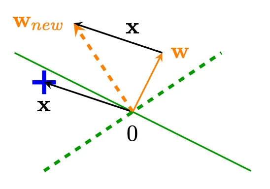
What does a perceptron update do?
Given y ∈ { 1 , − 1 } y \in \{1, -1\} y ∈ { 1 , − 1 }
w ← w + y ( i ) x ( i ) ← w ± x ( i ) \begin{align*}
w &\leftarrow w + y^{(i)}x^{(i)} \\
&\leftarrow w \pm x^{(i)}
\end{align*} w ← w + y ( i ) x ( i ) ← w ± x ( i )
Update of w w w y ( i ) x ( i ) y^{(i)}x^{(i)} y ( i ) x ( i )
Bias is updated by y ( i ) y^{(i)} y ( i )
Mistake on positive sample (y = 1 y = 1 y = 1 w ⊺ x ≤ 0 w^\intercal x \le 0 w ⊺ x ≤ 0
Increase the new weight w n e w w_{new} w n e w
w n e w ⊺ x = ( w + x ) ⊺ x = w ⊺ x + x ⊺ x > w ⊺ x \begin{align*}
w^\intercal_{new} x &= (w + x)^\intercal x \\
&= w^\intercal x + x^\intercal x \\
&> w^\intercal x
\end{align*} w n e w ⊺ x = ( w + x ) ⊺ x = w ⊺ x + x ⊺ x > w ⊺ x Mistake on negative sample (y = − 1 y = -1 y = − 1 w ⊺ x ≥ 0 w^\intercal x \ge 0 w ⊺ x ≥ 0
Decrease the new weight w n e w w_{new} w n e w
w n e w ⊺ x = ( w − x ) ⊺ x = w ⊺ x − x ⊺ x < w ⊺ x \begin{align*}
w_{new}^\intercal x &= (w - x)^\intercal x \\
&= w^\intercal x - x^\intercal x \\
&< w^\intercal x
\end{align*} w n e w ⊺ x = ( w − x ) ⊺ x = w ⊺ x − x ⊺ x < w ⊺ x How often can a perceptron misclassify a point x repeatedly
Assume K K K
y ( w + k y x ) ⊺ x ≤ 0 ⇒ y ( w ⊺ x ) + k ∣ ∣ x ∣ ∣ 2 ≤ 0 ⇒ k ∣ ∣ x ∣ ∣ 2 ≤ − y ( w ⊺ x ) ⇒ k ≤ − y ( w ⊺ x ) / ∣ ∣ x ∣ ∣ 2 \begin{align*}
&y(w + kyx)^\intercal x \le 0 \\
&\Rightarrow y(w^\intercal x) + k ||x||^2 \le 0 \\
&\Rightarrow k ||x||^2 \le -y(w^\intercal x) \\
&\Rightarrow k \le -y(w^\intercal x) / ||x||^2
\end{align*} y ( w + k y x ) ⊺ x ≤ 0 ⇒ y ( w ⊺ x ) + k ∣∣ x ∣ ∣ 2 ≤ 0 ⇒ k ∣∣ x ∣ ∣ 2 ≤ − y ( w ⊺ x ) ⇒ k ≤ − y ( w ⊺ x ) /∣∣ x ∣ ∣ 2 Perceptron Performance
∃ w ∗ \exist w^* ∃ w ∗
y ( i ) ( w ∗ ⊺ ) x ( i ) > 0 , ∀ ( x ( i ) ) , y ( i ) ∈ D y^{(i)}(w^{*\intercal})x^{(i)} > 0, \forall (x^{(i)}), y{(i)} \in D y ( i ) ( w ∗ ⊺ ) x ( i ) > 0 , ∀ ( x ( i ) ) , y ( i ) ∈ D
Rescale w ∗ w^* w ∗
∙ ∣ ∣ w ∗ ∣ ∣ = 1 ∙ ∣ ∣ x ( i ) ∣ ∣ ≤ 1 , ∀ x ( i ) ∈ D \begin{align*}
&\bullet ||w^*|| = 1 \\
&\bullet ||x^{(i)}|| \le 1, \forall x^{(i)} \in D
\end{align*} ∙ ∣∣ w ∗ ∣∣ = 1 ∙ ∣∣ x ( i ) ∣∣ ≤ 1 , ∀ x ( i ) ∈ D
Margin of a hyperplane γ \gamma γ
min ∣ w ∗ T x ( i ) ∣ , ∀ x ( i ) ∈ D \min|w^{*T}x^{(i)}|, \forall x^{(i)} \in D min ∣ w ∗ T x ( i ) ∣ , ∀ x ( i ) ∈ D
Formal Definition: Margin
γ = m a r g i n ( D , w ) = { min ( x , y ) ∈ D y ( w ⋅ x ) if w separates D − ∞ otherwise \gamma = margin(\mathbf{D}, w) = \begin{cases}
\min_{(x,y) \in \mathbf{D}} y(w \cdot x) & \text{if } w \text{ separates } \mathbf{D} \\
-\infty & \text{otherwise}
\end{cases} γ = ma r g in ( D , w ) = { min ( x , y ) ∈ D y ( w ⋅ x ) − ∞ if w separates D otherwise
Margin of a data set
The margin of dataset D is the supremum (maximum) over all possible weight vectors w of the margin function.”
In this case maximum and supremum only differ when m a r g i n ( D , w ) margin(\mathbf{D}, w) ma r g in ( D , w ) − ∞ -\infty − ∞
γ D = sup w , b { m a r g i n ( D , w ) } \gamma_D = \sup_{w, b}\{margin(\mathbf{D, w)}\} γ D = w , b sup { ma r g in ( D , w ) }
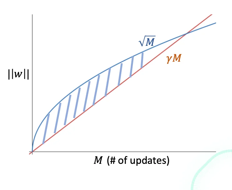
If all the conditions above hold, the perceptron algorithm makes at most
1 γ 2 \frac{1}{\gamma^2} γ 2 1 updates.
Proof
Given that:
y w ⊺ x ≤ 0 yw^\intercal x \le 0 y w ⊺ x ≤ 0 x x x w w w y w ∗ ⊺ x > 0 yw^{*\intercal} x > 0 y w ∗ ⊺ x > 0 w ∗ w^* w ∗
∙ \bullet ∙ w ⊺ w ∗ : w^\intercal w^*: w ⊺ w ∗ :
For each update, w ⊺ w ∗ w^\intercal w^* w ⊺ w ∗ γ \gamma γ
w n e w ⊺ w ∗ = ( w + y x ) ⊺ w ∗ = w ⊺ w ∗ + y w ∗ ⊺ x ∵ s i g n ( y ) = s i g n ( w ∗ ⊺ x ) ∵ y w ∗ T x = ∣ w ∗ ⊺ x ∣ ≥ γ ≥ w ⊺ w ∗ + γ ( ∵ y w ∗ ⊺ x ≥ γ ) \begin{align*}
w_{new}^\intercal w^* &= (w + yx)^\intercal w^* \\
&= w^{\intercal}w^* + yw^{*\intercal}x \\
&\because sign(y) = sign(w^{*\intercal} x) \\
&\because yw^{*T}x = |w^{*\intercal}x| \ge \gamma \\
&\ge w^\intercal w^* + \gamma \quad (\because yw^{*\intercal}x \ge \gamma)
\end{align*} w n e w ⊺ w ∗ = ( w + y x ) ⊺ w ∗ = w ⊺ w ∗ + y w ∗ ⊺ x ∵ s i g n ( y ) = s i g n ( w ∗ ⊺ x ) ∵ y w ∗ T x = ∣ w ∗ ⊺ x ∣ ≥ γ ≥ w ⊺ w ∗ + γ ( ∵ y w ∗ ⊺ x ≥ γ ) ∙ \bullet ∙ w ⊺ w : w^{\intercal}w: w ⊺ w :
For each update, w ⊺ w w^\intercal w w ⊺ w 1 1 1
w n e w ⊺ w n e w = ( w + y x ) ⊺ ( w + y x ) = w ⊺ w + 2 y w ⊺ x + y 2 x ⊺ x ≤ w ⊺ w + 1 ( ∵ y w T x ≤ 0 , x ⊺ x ≤ 1 ) \begin{align*}
w_{new}^\intercal w_{new} &= (w + yx)^\intercal (w + yx)\\
&= w^\intercal w + 2yw^\intercal x + y^2x^\intercal x \\
&\le w^\intercal w + 1 \quad (\because yw^Tx \le 0,\ x^\intercal x \le 1)
\end{align*} w n e w ⊺ w n e w = ( w + y x ) ⊺ ( w + y x ) = w ⊺ w + 2 y w ⊺ x + y 2 x ⊺ x ≤ w ⊺ w + 1 ( ∵ y w T x ≤ 0 , x ⊺ x ≤ 1 ) ∙ \bullet ∙ M γ ≤ w T w ∗ = ∣ w T w ∗ ∣ ≤ ∣ ∣ w ∣ ∣ ⋅ ∣ ∣ w ∗ ∣ ∣ (Cauchy-Schwarz Inequality) = ∣ ∣ w ∣ ∣ ⋅ 1 (since ∣ ∣ w ∗ ∣ ∣ = 1 ) = ∣ ∣ w ∣ ∣ = w ⊺ w ≤ M (by the effect of an update on w ⊺ w ) ⇒ M γ ≤ M ⇒ M 2 γ 2 ≤ M ⇒ M ≤ 1 γ 2 \begin{align*}
M\gamma &\leq w^T w^* \\
&= |w^T w^*| \\
&\leq ||w|| \cdot ||w^*|| \quad \text{(Cauchy-Schwarz Inequality)} \\
&= ||w|| \cdot 1 \quad \text{(since } ||w^*|| = 1\text{)} \\
&= ||w|| \\
&= \sqrt{w^\intercal w} \\
&\le \sqrt{M} \quad \text{(by the effect of an update on } w^\intercal w) \\
&\Rightarrow M\gamma \le \sqrt{M} \\
&\Rightarrow M^2\gamma^2 \le M \\
&\Rightarrow M \le \frac{1}{\gamma^2}
\end{align*} M γ ≤ w T w ∗ = ∣ w T w ∗ ∣ ≤ ∣∣ w ∣∣ ⋅ ∣∣ w ∗ ∣∣ (Cauchy-Schwarz Inequality) = ∣∣ w ∣∣ ⋅ 1 (since ∣∣ w ∗ ∣∣ = 1 ) = ∣∣ w ∣∣ = w ⊺ w ≤ M (by the effect of an update on w ⊺ w ) ⇒ M γ ≤ M ⇒ M 2 γ 2 ≤ M ⇒ M ≤ γ 2 1
Improved Generalization: Voting and Averaging
The key issue of the initial perceptron is that it counts later points more than it counts earlier points.
Give more say to weight vectors that survive long enough
Voted Perceptron
Each weight vector has its own counter for survival times
w ( 1 ) , … , w ( k ) w^{(1)},\ \dots,\ w^{(k)} w ( 1 ) , … , w ( k ) K + 1 K + 1 K + 1 w 0 w_0 w 0 c ( 1 ) , … , c ( k ) c^{(1)},\ \dots,\ c^{(k)} c ( 1 ) , … , c ( k )
y ^ = s i g n ( ∑ k = 1 K c ( k ) × s i g n ( w ( k ) ⋅ x ^ ) ) \hat{y} = sign(\sum_{k=1}^{K} c^{(k)} \times sign(w^{(k)} \cdot \hat{x})) y ^ = s i g n ( k = 1 ∑ K c ( k ) × s i g n ( w ( k ) ⋅ x ^ )) Averaged Perceptron
At test time, you predict according to the average weight vector rather than the voting.
y ^ = s i g n ( ∑ k = 1 K c ( k ) × ( w ( k ) ⋅ x ^ ) ) = s i g n ( ∑ k = 1 K c ( k ) × ( w ( k ) ) ⋅ x ^ ) \begin{align*}
\hat{y} &= sign(\sum_{k=1}^{K} c^{(k)} \times (w^{(k)} \cdot \hat{x})) \\
&= sign(\sum_{k=1}^{K} c^{(k)} \times (w^{(k)}) \cdot \hat{x}) \\
\end{align*} y ^ = s i g n ( k = 1 ∑ K c ( k ) × ( w ( k ) ⋅ x ^ )) = s i g n ( k = 1 ∑ K c ( k ) × ( w ( k ) ) ⋅ x ^ ) Algorithm
AveragedPerceptronTrain ( D , M a x I t e r ) 1 : w d ← ⟨ 0 ⃗ , … , 0 ⃗ ⟩ // initialize weights 2 : u ⟨ 0 ⃗ , … , 0 ⃗ ⟩ // initialize cached weights 3 : for i t e r = 1 … M a x I t e r do 4 : for all ( x , y ) ∈ D do 5 : if y ( w ⋅ x ) ≤ 0 ⃗ t h e n 6 : w ← w + y x 5 : u ← u + y c x 9 : end if 9 : c ← c + 1 10 : end for 11 : end for 12 : return w − 1 c u \begin{array}{l}
\hline
{\text{AveragedPerceptronTrain}}(D, MaxIter) \\
\hline
\begin{array}{ll}
1: & w_d \leftarrow \langle\vec{\scriptstyle 0},\ \dots,\ \vec{\scriptstyle 0}\rangle& \text{// initialize weights} \\
2: & u \langle \vec{\scriptstyle 0},\ \dots,\ \vec{\scriptstyle 0}\rangle& \text{// initialize cached weights} \\
3: & \textbf{for } iter = 1 \ldots MaxIter \textbf{ do} \\
4: & \quad \textbf{for all } (x,y) \in D \textbf{ do} \\
5: & \quad \textbf{if } y(w \cdot x) \le \vec{\scriptstyle 0}\ then\\
6: & \quad \quad w \leftarrow w + yx \\
5: & \quad \quad u \leftarrow u + ycx \\
9: & \quad \quad \textbf{end if} \\
9: & \quad c \leftarrow c + 1 \\
10: & \quad \textbf{end for} \\
11: & \textbf{end for} \\
12: & \textbf{return } w - \frac{1}{c} u \\ \\
\end{array} \\
\hline
\end{array} AveragedPerceptronTrain ( D , M a x I t er ) 1 : 2 : 3 : 4 : 5 : 6 : 5 : 9 : 9 : 10 : 11 : 12 : w d ← ⟨ 0 , … , 0 ⟩ u ⟨ 0 , … , 0 ⟩ for i t er = 1 … M a x I t er do for all ( x , y ) ∈ D do if y ( w ⋅ x ) ≤ 0 t h e n w ← w + y x u ← u + yc x end if c ← c + 1 end for end for return w − c 1 u // initialize weights // initialize cached weights