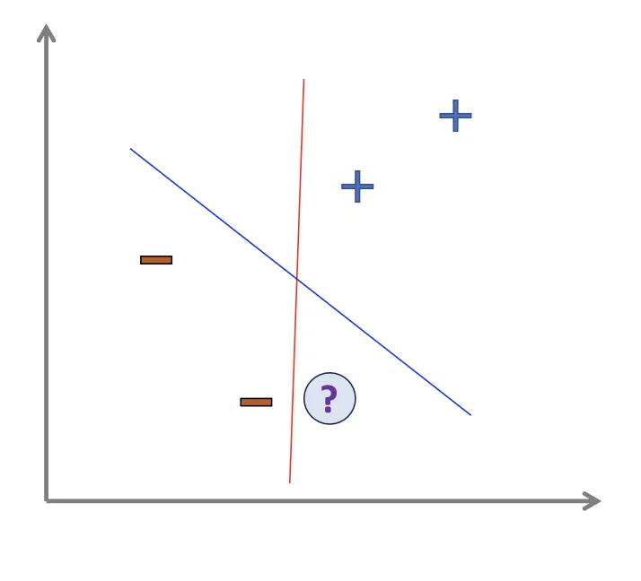
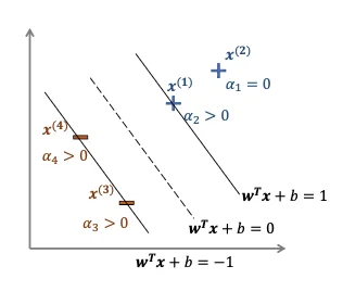
Sometimes, we may have multiple decision boundaries.
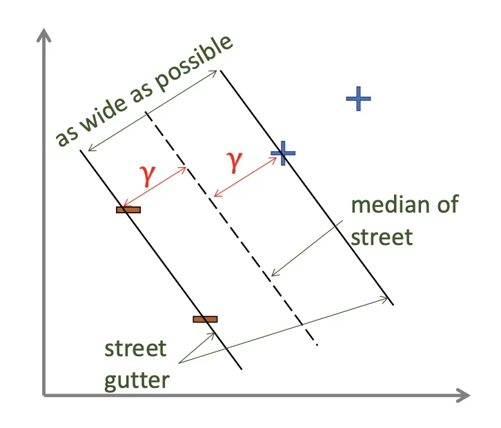
Maximizing the margin
γ: The distance between a data point to the decision boundary
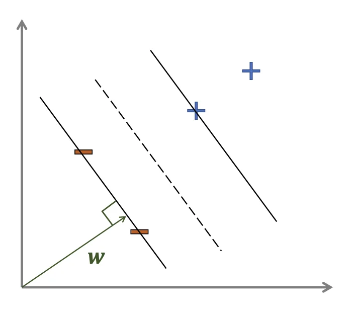
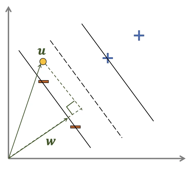
Decision Rule
Hyperplane
H={x:w⊺x+b=0}
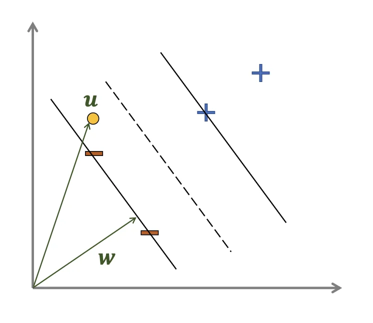
w
a vector perpendicular to the median line
u
an unknown example
w⊺u≥−b
Project u onto w
{positive(w⊺u+b≥0)negative(otherwise)
How to calculate w and b?
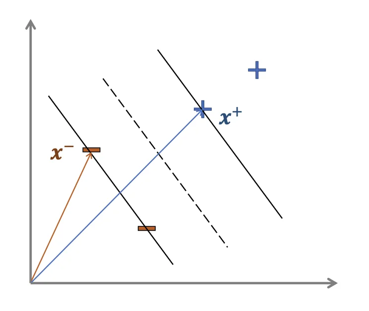
Add more constraints
w⊺x++b≥aw⊺x−+b≤−aLet y be an activation functiony={+1(for positive sample)−1(for negative sample)y+(w⊺x++b)≥ay−(w⊺x−+b)≥a⟹y(i)(w⊺x(i)+b)≥ay(i)(w⊺x(i)+b)=a( for x(i) in gutter)
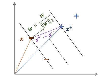
Width of the Street
Given that y(i)(w⊺x(i)+b)=a for x in gutter
w=∣∣w∣∣2w⊺(x+−x−)∵(x+ and x− are both in the gutter)∴w⊺x+=a−b,w⊺x−=−a−b=∣∣w∣∣22aa,bmax∣∣w∣∣22a⟹w,bmax∣∣w∣∣22a⟹w,bmax∣∣w∣∣2a⟹w,bmina∣∣w∣∣2s.t.y(i)(w⊺x(i)+b)≥a
Since a is arbitrary, can normalize equations by a
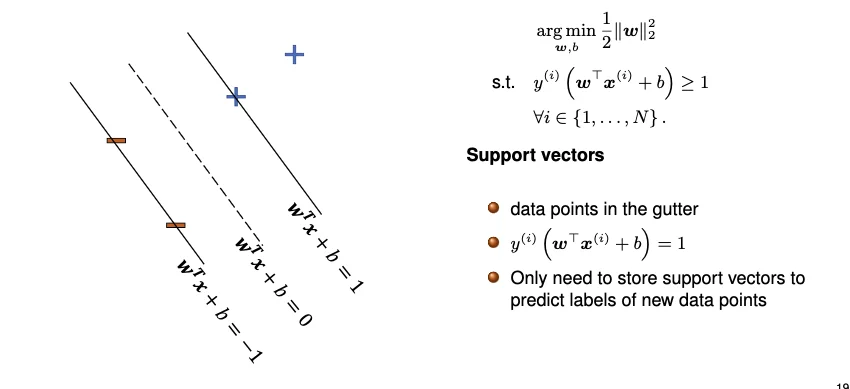
w,bmin21∣∣w∣∣22,s.t.y(i)(w⊺x(i)+b)≥1
Support Vectors
lies in:
{w⊺x+b=1w⊺x+b=−1
Under the KKT condition, only a few αi can be non-zero
αi∗gi(w∗)=0,i=1,…,N
where
gi(w∗)=1−y(i)(w⊺x(i)+b)
Training data are called support vectors if their αi are non-zero
∵
only a few αi can be non-zero
y(i)(w⊺x(i)+b)=1 when αi is non-zero
∴
b=y(t)−w⊺x(t)(αt>0)
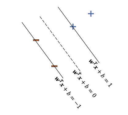
Hard Margin SVM
Assume that data are linearly separable
w,bargmin21∣∣w∣∣22s.t.y(i)(w⊺x(i)+b)≥1
This is a convex quadratic programming problem with linear constraints
Tip
What is Quadratic Programming?
A type of mathematical optimization problem
Similar to linear programming but minimizes a quadratic function
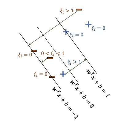
Soft Margin SVM
In real-world data, there may be:
Overlapping classes
Noisy points
Outliers
Assume that data are non-linearly separable
Introduce a trade-off parameter between error and margin and slack variables to measure how much a point violates the margin constraint
Bias term:
For any support vector xt with 0<αt∗<C:
b∗=yt−j∑αj∗yjK(xj,xt)
If multiple margin SVs exist, take the average b∗.
KKT Conditions (Soft-Margin)
Condition
Mathematical Form
Meaning in SVM
Stationarity
w=∑iαiyixi, ∑iαiyi=0, C−αi−μi=0
Gradient equilibrium
Primal Feasibility
yi(w⊤xi+b)≥1−ξi, ξi≥0
Must satisfy primal constraints
Dual Feasibility
αi≥0, μi≥0
Non-negative multipliers
Complementary Slackness
αi[1−ξi−yi(w⊤xi+b)]=0, μiξi=0
Active constraints ↔ positive multipliers
Intepretation
Condition
yif(xi)
Classification
Margin Status
Slack Variable ξi
Interpretation
Outside margin
>1
✅ Correct
Outside margin
ξi=0
Confidently correct (no penalty)
On margin
=1
✅ Correct
On boundary
ξi=0
Support vector (defines margin)
Inside margin (correct side)
0<yif(xi)<1
✅ Correct
Inside margin
0<ξi<1
Correct but too close to boundary (penalized)
Misclassified (wrong side)
yif(xi)<0
❌ Incorrect
Inside margin (wrong side)
ξi>1
Misclassified (heavily penalized)
Final Decision Function
Linear Case:
f(x)=sign(i∑αi∗yixi⊤x+b∗)
Kernelized Case:
f(x)=sign(i∑αi∗yiK(xi,x)+b∗)
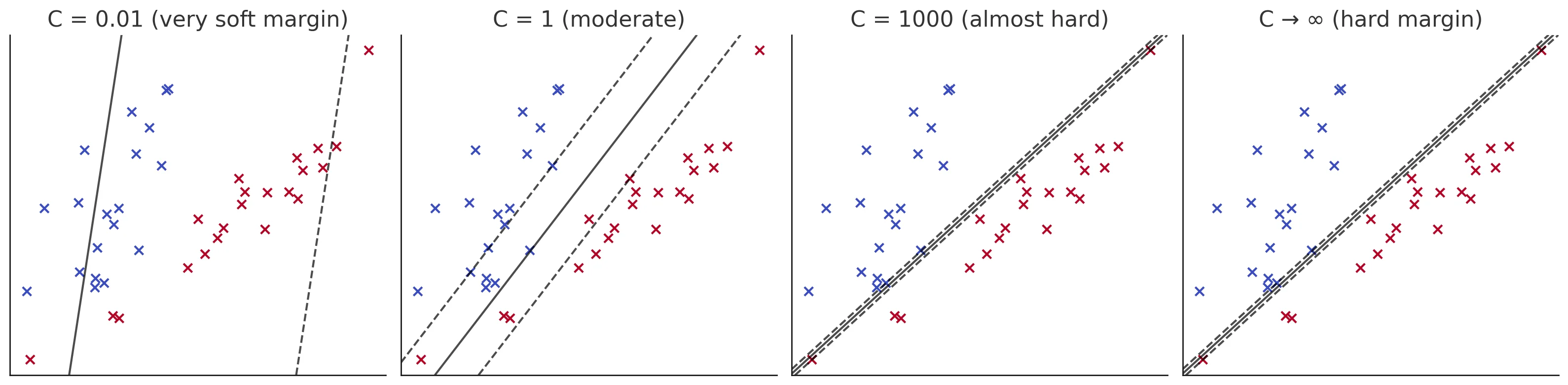
Margin and Limit Behavior
Margin width:∥w∗∥2
As C→∞: Soft-margin SVM → Hard-margin SVM (if data are separable)
As C→0: Margin dominates, high tolerance for error (underfitting)
Intuitive Summary
Hard-Margin: No misclassification; all points must be correctly separated.
Soft-Margin: Allows some violations; balances accuracy and generalization via C.
Support Vectors: Points with αi>0 define the decision boundary.
Dual Form: Enables kernel trick; optimization depends only on dot products or K(xi,xj).
Implementation
Helper
defpoly_implementation(x, y, degree):assert x.size()== y.size(),'The dimensions of inputs do not match!'with torch.no_grad():return(1+(x * y).sum()).pow(degree)defpoly(degree):returnlambda x, y: poly_implementation(x, y, degree)defrbf_implementation(x, y, sigma):assert x.size()== y.size(),'The dimensions of inputs do not match!'with torch.no_grad():return(-(x - y).norm().pow(2)/2/ sigma / sigma).exp()defrbf(sigma):returnlambda x, y: rbf_implementation(x, y, sigma)defxor_data():
x = torch.tensor([[1,1],[-1,1],[-1,-1],[1,-1]], dtype=torch.float)
y = torch.tensor([1,-1,1,-1], dtype=torch.float)return x, y
SVM
defsvm_solver(
x_train, y_train, lr, num_iters, kernel=hw3_utils.poly(degree=1), c=None):"""
Computes an SVM given a training set, training labels, the number of
iterations to perform projected gradient descent, a kernel, and a trade-off
parameter for soft-margin SVM.
Arguments:
x_train: 2d tensor with shape (N, d).
y_train: 1d tensor with shape (N,), whose elememnts are +1 or -1.
lr: The learning rate.
num_iters: The number of gradient descent steps.
kernel: The kernel function.
The default kernel function is 1 + <x, y>.
c: The trade-off parameter in soft-margin SVM.
The default value is None, referring to the basic, hard-margin SVM.
Returns:
alpha: a 1d tensor with shape (N,), denoting an optimal dual solution.
Initialize alpha to be 0.
Return alpha.detach() could possibly help you save some time
when you try to use alpha in other places.
"""# TODO
N = x_train.shape[0]
alpha = torch.zeros(N, requires_grad=True)
Y = torch.diag(y_train)# Build the kernel beforehand
K = create_kernel(x_train, x_train, N, N, kernel)for _ inrange(num_iters):# The matrix form of the original dual problem: sum(alpha) - alpha^T(YKY)alpha
L = alpha.sum()-0.5* alpha @ (Y @ K @ Y) @ alpha
L.backward()# update alphawith torch.no_grad():
alpha += lr * alpha.grad
# clamp the rangeif c:
alpha = torch.clamp_(
alpha,min=0,max=c,)else:
alpha = torch.clamp_(
alpha,min=0,)
alpha.grad.zero_()
alpha.requires_grad_()return alpha.detach()defsvm_predictor(alpha, x_train, y_train, x_test, kernel=hw3_utils.poly(degree=1)):"""
Returns the kernel SVM's predictions for x_test using the SVM trained on
x_train, y_train with computed dual variables alpha.
Arguments:
alpha: 1d tensor with shape (N,), denoting an optimal dual solution.
x_train: 2d tensor with shape (N, d), denoting the training set.
y_train: 1d tensor with shape (N,), whose elements are +1 or -1.
x_test: 2d tensor with shape (M, d), denoting the test set.
kernel: The kernel function.
The default kernel function is 1 + <x, y>.
Return:
A 1d tensor with shape (M,), the outputs of SVM on the test set.
"""
N = x_train.shape[0]
M = x_test.shape[0]
K_train = create_kernel(x_train, x_train, N, N, kernel)
K_test = create_kernel(x_train, x_test, N, M, kernel)
support_idx = torch.where(alpha > _EPS)[0]iflen(support_idx)==0:return torch.zeros(M)
min_alpha_idx = support_idx[torch.argmin(alpha[support_idx])]# y_support - \sum^{N}_{j = 1} \alpha_j * y_j * K(x_j, x_k)
b = y_train[min_alpha_idx]-(alpha * y_train * K_train[:, min_alpha_idx]).sum()# Compute predictions: f(x) = \sum_{i=1}^{N} \alpha_i * y_i * K(x_i, x) + b
f = torch.sum((alpha * y_train).unsqueeze(1)* K_test, dim=0)+ b
return torch.sign(f)