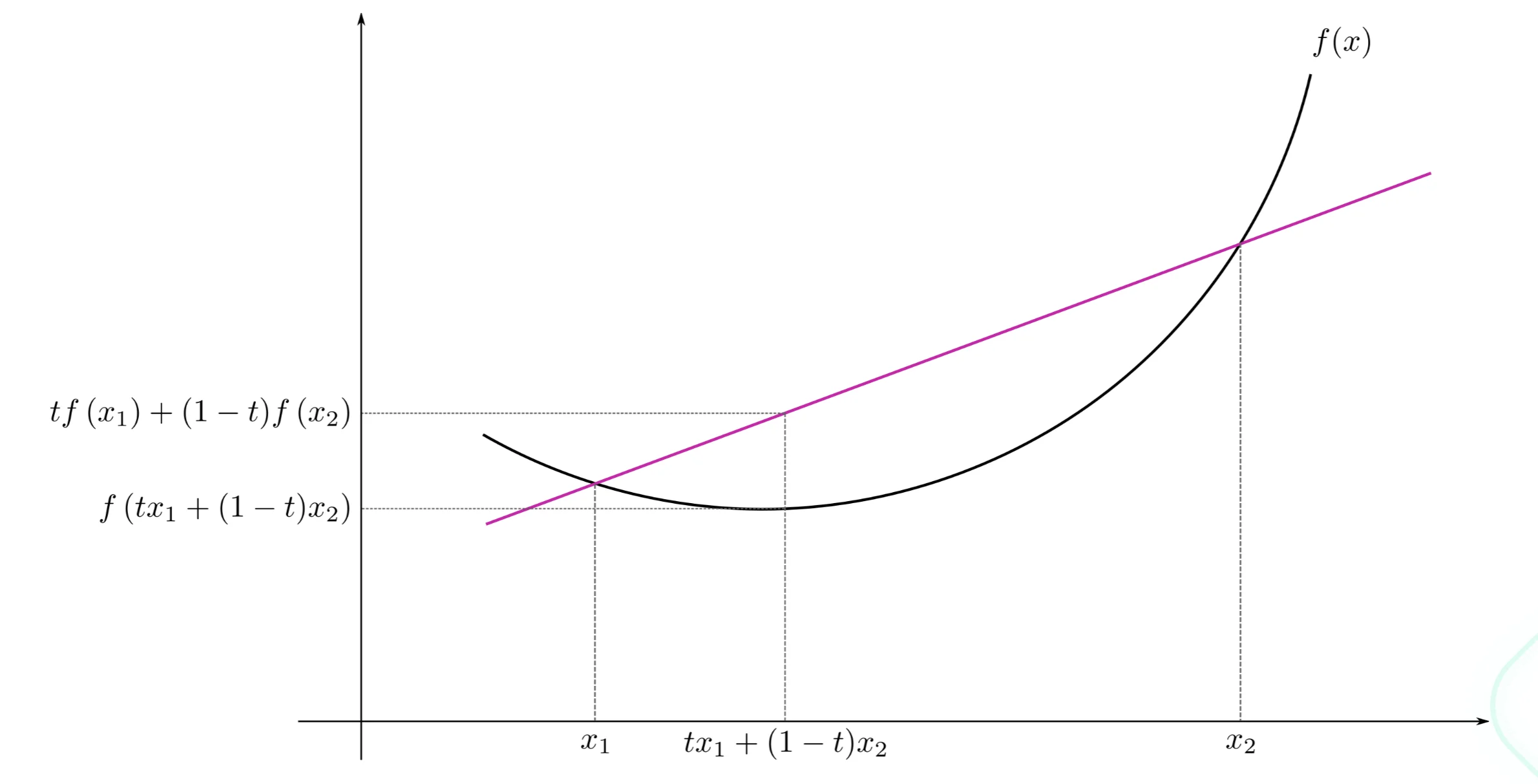
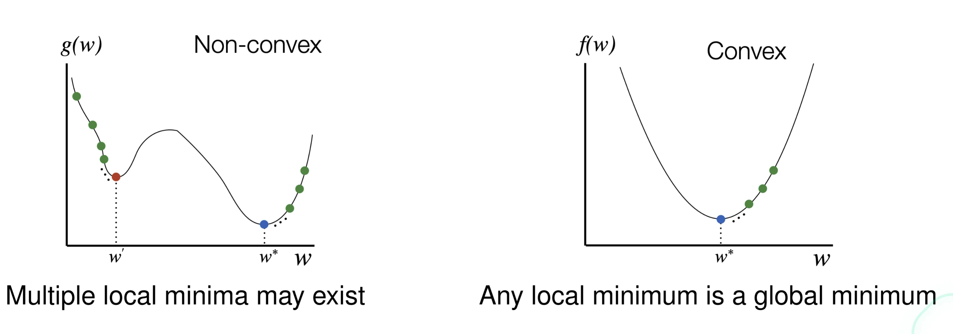
Minimize a convex, continuous and differentiable function
Taylor Expansion
ℓ(w+s)≈ℓ(w)+g(w)⊺s
where
g(w)=∇ℓ(w) is the gradient
l(w+s)≈ℓ(w)+g(w)⊺s+21s⊺H(w)s
where
H(w)=∇2ℓ(w) is the Hessian of ℓ
Gradient Descent
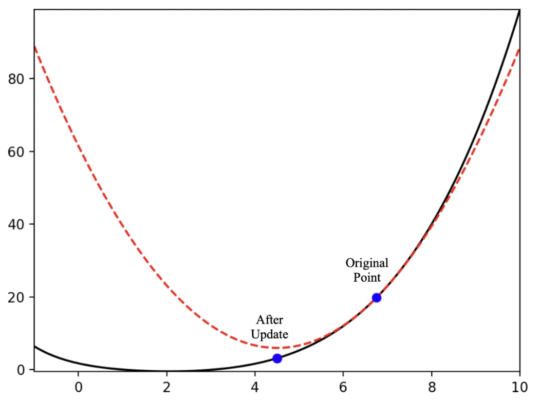
Use the first order approximation
Assume that the function ℓ around w is linear and behaves like ℓ(w)+g(w)⊺s
Find a vector s that minimized ℓ
s=−αg(w)
for some small α as the learning rate
After one update
ℓ(w+(−αg(w)))≈ℓ(w)−>0αg(w)⊺g(w)<ℓ(b)
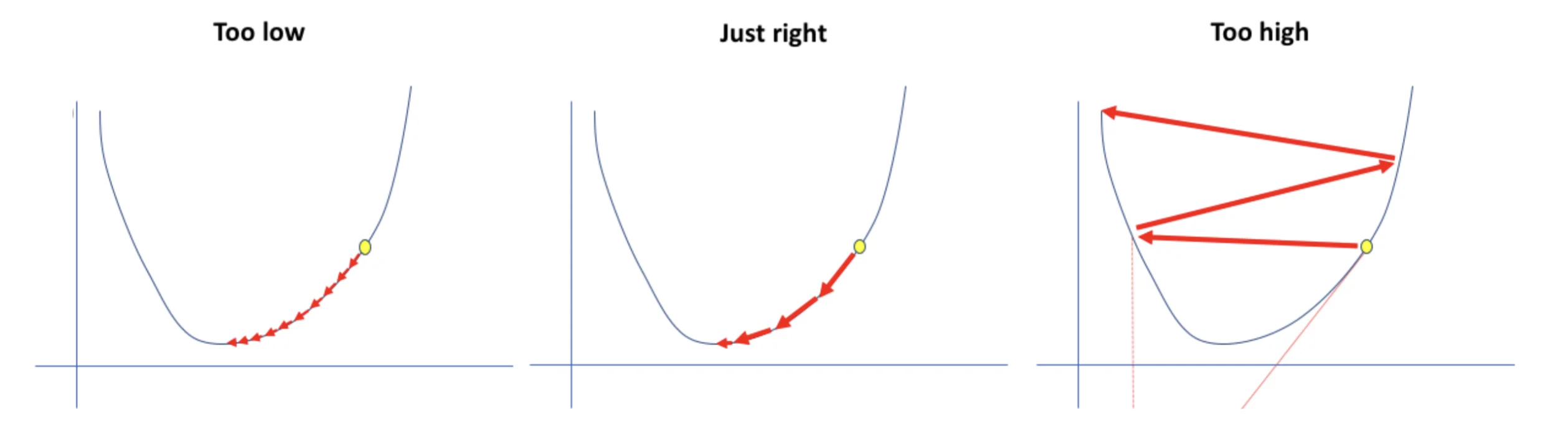
Choosing the step
A safe choice is to set α=tc
c: some constant
t: the number of updates taken
Guarantees that the gradient descent eventually become small enough to converge
Types
∙ Batch Gradient
use error over the entire training set D
Do until satisfied:
Compute the graident: ∇ℓD(w)Update the vector of parameters: w←w−α∇ℓD(w)
∙ Stochastic Gradient
use error over a single training example from D
Do until satisfied:
Choose (with replacement) a random training example(x(i),y(i))∈DCompute the graident just for them: ∇ℓ(x(i),y(i))(w)Update the vector of parameters: w←w−α∇ℓ(x(i),y(i))(w)
Tip
Stochastic approximates Batch arbitrarily closely as α→0
Stochastic can be much faster when D is very large
Interemediate approach: use error over subsets of D
Gradient descent is slow when it is close to minimum