9. Bias Variance

Training Data

• $\mathcal{D} = \{(x^{(i)}, y^{(i)})\}_{i = 1}^N$
• drawn i.i.d. from some distribution $(X, Y)$
• Assume a regression setting, $Y \in \R$
• For a given $x$, there may be many $y$
• Different features may have different labels
• $x^{(i)}_j$ in $x^{(i)}$ may not have the same $y^{(i)}$

Expected Label (given $x \in \R^d$)

• For a given $x \in \R^d$, the expected label:

Expected Test Error (given $h_D$)

• Now, we have some ML Algorithm ($\mathcal{A}$), which takes the dataset $\mathcal{D}$ as an input to generate the predictor $h_\mathcal{D}$

• With the predictor $h_\mathcal{D}$, we can hopefully derive the expected test error as follows:

Expected Predictor (given $\mathcal A$)

• Assume that:
• $\mathcal A:$ Linear regression
• $\mathcal D:$ Sales data from the previous year
• $h_\mathcal D:$ A random variable
• Expected Predictor Given A

Expected Test Error (given $\mathcal A$)

Full Derivation

1. Rewrite the formula by plugging $\bar{h}$ in

2. Solve for $\mathbb{E}_{x, y, \mathcal D} [(h_\mathcal D(x) - \bar{h}(x))(\bar{h}(x) - y)]$

3. Solve for $\mathbb{E}_{x, y} [(\bar{h}(x) - y)^2]$

4. Solve for $\mathbb{E}_{x, y}[(\bar{h}(x) - \bar{y}(x))(\bar{y}(x) - y)]$

5. Plug all the solved equations in:

Breaking Down the Expected Test Error

The expected test error equals

• Variance (due to data randomness)
• Bias (due to model misspecification)
• Irreducible noise (due to inherent randomness in data).

1. Expected Test Error

• This is the overall expected test error — how far the model’s predictions $h_{\mathcal{D}}(x)$ are from the true values $y$, averaged over:
• all possible datasets $\mathcal{D}$ you could have trained on,
• all possible inputs $x$, and
• all possible outputs $y$ drawn from the true data distribution.

2. First term:

• This measures how much the predictions from different datasets fluctuate around their average prediction $\bar{h}(x)$.
• In words:
• variance
• how sensitive the model is to the particular training data it saw.
• If this term is large, your model changes a lot depending on the training data (i.e., it’s unstable or overfits).
• If it’s small, your model is consistent across different datasets.

3. Second term:

• irreducible
• we may add some more data to resovle this issue
• This measures how far the model’s average prediction $\bar{h}(x)$ is from the best expected output $\bar{y}(x) = \mathbb{E}_{y \mid x}[Y]$.
• In words:
• bias
• the systematic error of your model.
• If your model’s structure can’t capture the true relationship, this term is large (underfitting).
• If it’s small, your model’s mean prediction is close to the truth.

4. Third term:

• This measures how much the true data itself varies around its expected value.
• In words:
• irreducible noise
• randomness or natural variability in the data that no model can ever predict perfectly.

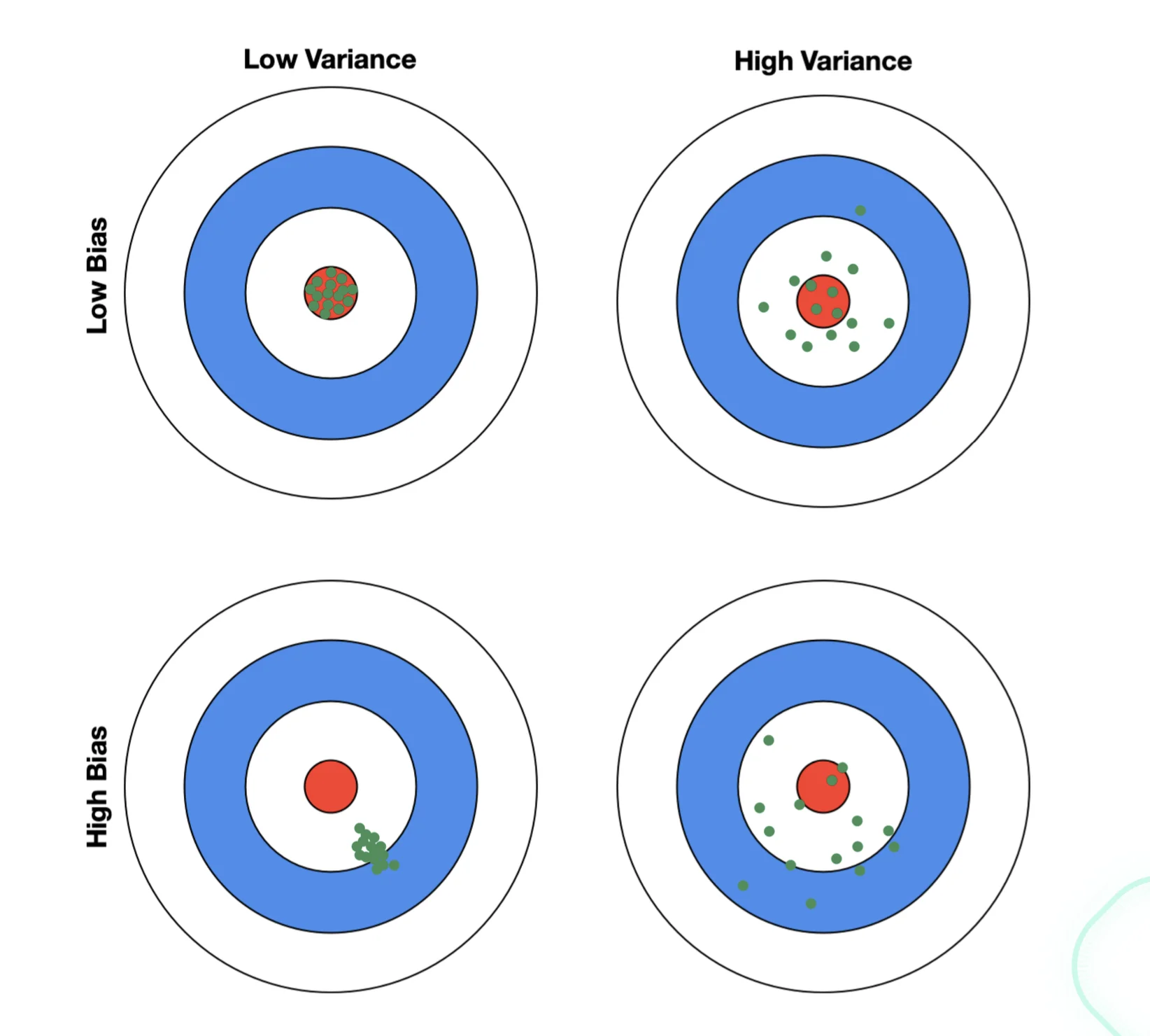
Illustration of Bias and Variance