4. Central Limit Theorem

In progress

Sep 25, 2025

#Math #Statistics

On this page

The Law of Large Numbers
Definition
Proof
Diagram Comparison

The Law of Large Numbers

Definition

Given
- random variables $X_1, X_2, \dots, X_n$ that are $i.i.d.$
- $\mathbb{E}[X] = \mu$
- $\mathbb{V}[X] = \sigma^2$
According to the Law of Large Numbers

\bar{X}_n = \frac{1}{n} \sum_{i = 1}^{n} X_i \;\xrightarrow{\mathbb{P}}\; \mu \quad (n \to \infty)

Proof

Let an event $A \in \{0,1\}$ , where $P(A = 1) = p$ and $P(A = 0) = q = 1 - p$ .
Consider $n$ independent trials of $A$ , and let $X$ be the number of times $A = 1$ occurs.
Then $X$ follows a binomial distribution:

\begin{align*} P(X = x) &= \binom{n}{x} p^{x} q^{\,n - x}, \\ \mu &= np, \\ \sigma^2 &= npq. \end{align*}

As $n \to \infty$ , with $p$ fixed and $x$ in a neighborhood of $np$ , the binomial distribution admits a normal approximation (de Moivre–Laplace theorem):

X \approx N(\mu, \sigma^2).

Under this approximation, the probability mass function of $X$ can be approximated by the probability density function:

f_X(x) = \frac{1}{\sqrt{2\pi\sigma^2}} \exp\!\left(-\frac{(x - \mu)^2}{2\sigma^2}\right).

Now define a new random variable

\bar X = \frac{X}{n},

representing the proportion of times $A = 1$ occurs in $n$ trials.

Using a change of variables under the normal approximation, where $x = n\bar x$ and $\frac{dx}{d\bar x} = n$ , we obtain:

\begin{align*} f_{\bar X}(\bar x) &= n \cdot f_X(n\bar x) \\ &= \frac{n}{\sqrt{2\pi npq}} \exp\!\left(-\frac{(n\bar x - np)^2}{2npq}\right) \\ &= \frac{1}{\sqrt{2\pi \frac{pq}{n}}} \exp\!\left(-\frac{(\bar x - p)^2}{2\frac{pq}{n}}\right). \end{align*}

Therefore, the mean and variance of $\bar X$ are:

\mu_{\bar X} = p, \qquad \sigma^2_{\bar X} = \frac{pq}{n}.

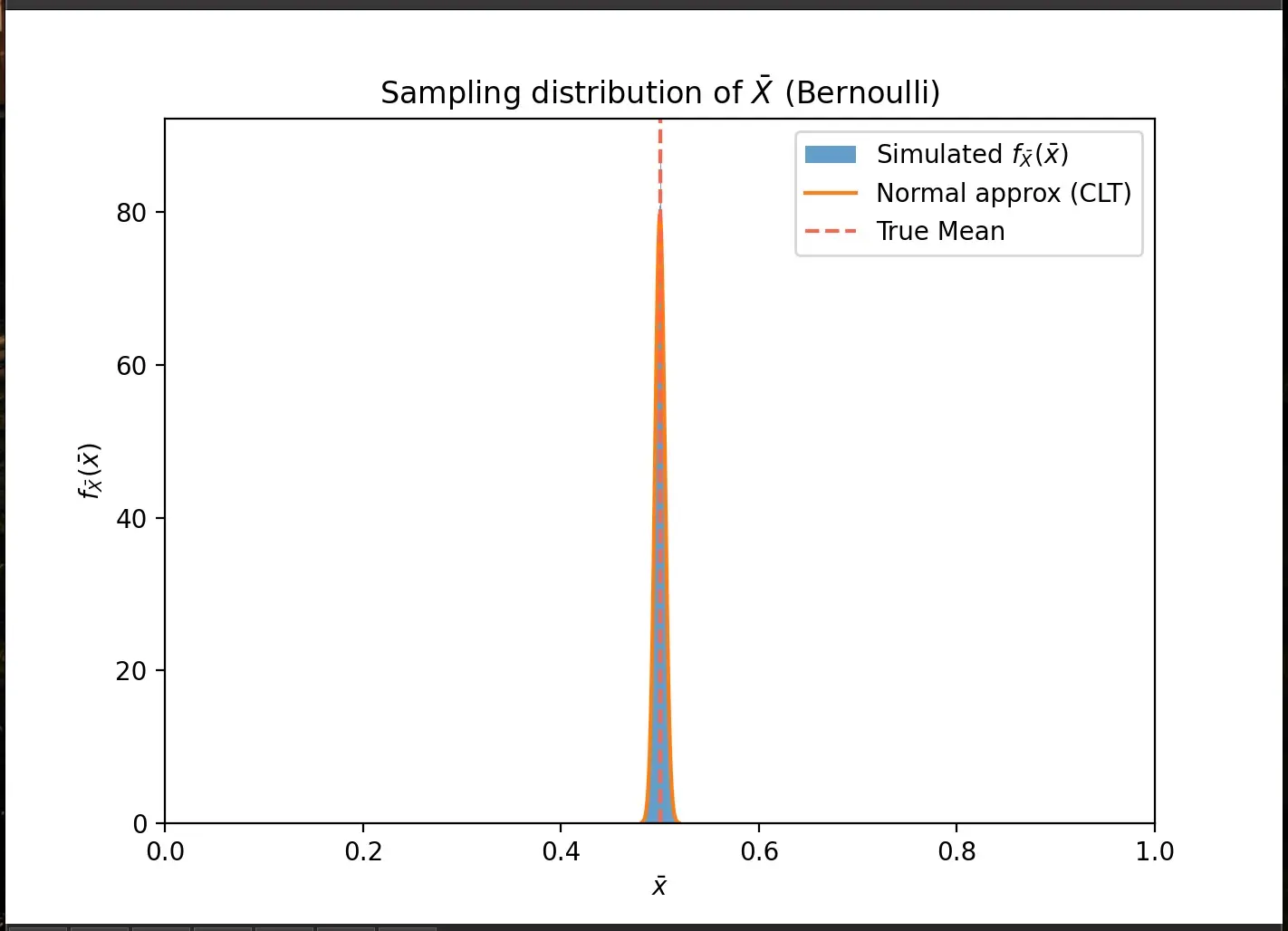
As $n \to \infty$ , the variance converges to zero:

\lim_{n \to \infty} \sigma^2_{\bar X} = \lim_{n \to \infty} \frac{pq}{n} = 0.

Hence, under the normal approximation, the distribution of $\bar X$ concentrates at $p$ and converges to a degenerate distribution at $p$ .
This implies that the sample proportion converges in probability to $p$ :

\lim_{n \to \infty} \frac{X}{n} = p.

Diagram Comparison

n = 30

n = 30

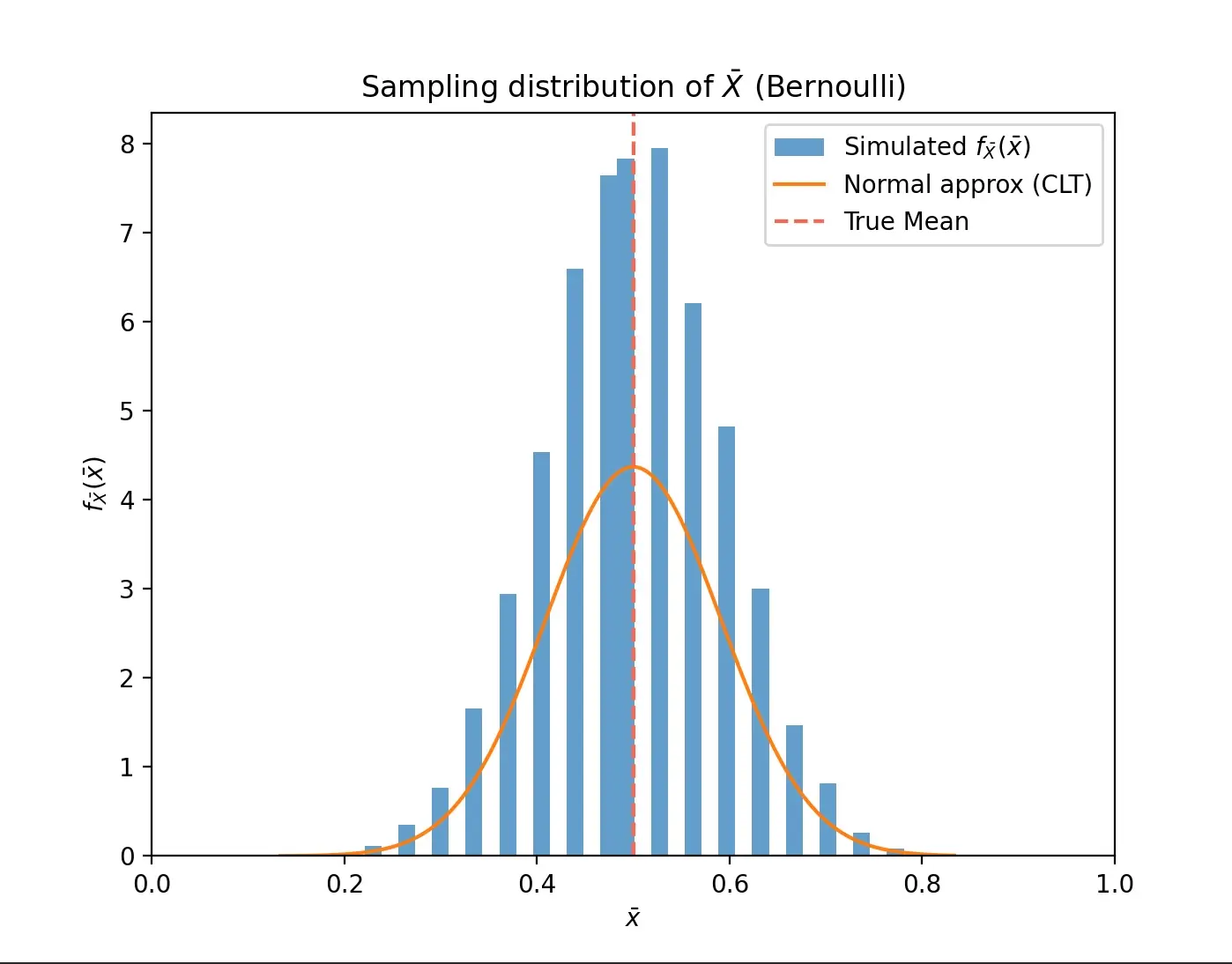
n = 10000

n = 10000