3. Naive Bayes
MLE and MAP
Components
Dataset D \mathcal{D} D : i.i.d (independent and identically distributed) drawn from some unknonw distributionP θ ( X , Y ) P_\theta(X, Y) P θ ( X , Y )
MLE (Maximum Likelihood Estimate)
Choose θ \theta θ D \mathcal{D} D
θ ^ M L E = arg max θ P ( D ∣ θ ) \hat{\theta}_{MLE} = \argmax_{\theta}P( \mathcal{D} | \theta) θ ^ M L E = θ arg max P ( D ∣ θ ) MAP (Maximum A Priori)
Choose θ \theta θ given prior proability and observed data .
θ ^ M A P = arg max θ P ( θ ∣ D ) = arg max θ P ( θ ) P ( D ∣ θ ) P ( D ) ∝ arg max θ P ( D ∣ θ ) P ( θ ) ( P ( D ) does not depend on θ ) \begin{align*}
\hat{\theta}_{MAP} &= \argmax_{\theta} P(\theta | \mathcal{D}) \\
&= \argmax_{\theta} \frac{P(\theta)P(\mathcal{D} | \theta)}{P(\mathcal{D})} \\
&\propto \argmax_{\theta} P(\mathcal{D} | \theta) P(\theta) \quad (P(\mathcal{D})\text{ does not depend on }\theta)
\end{align*} θ ^ M A P = θ arg max P ( θ ∣ D ) = θ arg max P ( D ) P ( θ ) P ( D ∣ θ ) ∝ θ arg max P ( D ∣ θ ) P ( θ ) ( P ( D ) does not depend on θ ) Example
A dataset D \mathcal{D} D α H \alpha_H α H α T \alpha_T α T
MLE (Exactly the frequency of head):
θ ^ M L E = arg max θ P ( D ∣ θ ) = α H α H + α T \begin{align*}
\hat{\theta}_{MLE} &= \argmax_{\theta}P( \mathcal{D}|\theta) \\
&= \frac{\alpha_H}{\alpha_H + \alpha_T}
\end{align*} θ ^ M L E = θ arg max P ( D ∣ θ ) = α H + α T α H θ ^ M A P = arg max θ P ( θ ∣ D ) = α H + β H − 1 ( α H + β H − 1 ) ( α T + β T − 1 ) \begin{align*}
\hat{\theta}_{MAP} &= \argmax_{\theta}P(\theta | \mathcal{D}) \\
&= \frac{\alpha_H + \beta_H - 1}{(\alpha_H + \beta_H - 1)(\alpha_T + \beta_T - 1)}
\end{align*} θ ^ M A P = θ arg max P ( θ ∣ D ) = ( α H + β H − 1 ) ( α T + β T − 1 ) α H + β H − 1
β H − 1 \beta_H - 1 β H − 1 β T − 1 \beta_T - 1 β T − 1
Example 2
D \mathcal{D} D P ( D ∣ θ ) P(\mathcal{D}|\theta) P ( D ∣ θ ) θ \theta θ { θ 1 , θ 2 , … , θ M } \{\theta_1, \theta_2, \dots, \theta_M\} { θ 1 , θ 2 , … , θ M }
P ( D ∣ θ ) ∝ θ 1 α 1 ⋅ θ 2 α 2 ⋯ θ M α M P(\mathcal{D} | \theta) \propto \theta^{\alpha_1}_1 \cdot \theta^{\alpha_2}_2 \cdots \theta^{\alpha_M}_M P ( D ∣ θ ) ∝ θ 1 α 1 ⋅ θ 2 α 2 ⋯ θ M α M
θ m \theta_m θ m
∙ \bullet ∙ Dirichlet Distribution is used in this case
P ( θ ) = θ 1 β 1 − 1 θ 2 β 2 − 1 ⋯ θ M β M − 1 B ( β 1 , … , B M ) ∼ D i r i c h l e t ( β 1 , … , β M ) P(\theta) = \frac{\theta^{\beta_1 - 1}_1\theta^{\beta_2 - 1}_2 \cdots \theta^{\beta_M - 1}_M}{B(\beta_1, \dots, B_M)} \sim Dirichlet(\beta_1, \dots, \beta_M) P ( θ ) = B ( β 1 , … , B M ) θ 1 β 1 − 1 θ 2 β 2 − 1 ⋯ θ M β M − 1 ∼ D i r i c h l e t ( β 1 , … , β M ) where B ( β 1 , … , B M ) B(\beta_1, \dots, B_M) B ( β 1 , … , B M )
∙ \bullet ∙ P ( θ ∣ D ) ∝ P ( D ∣ θ ) P ( θ ) ∼ D i r i c h l e t ( α 1 + β 1 , … , α M + β M ) P(\theta | \mathcal{D}) \propto P(\mathcal{D} | \theta) P(\theta) \sim Dirichlet(\alpha_1 + \beta_1, \dots, \alpha_M + \beta_M) P ( θ ∣ D ) ∝ P ( D ∣ θ ) P ( θ ) ∼ D i r i c h l e t ( α 1 + β 1 , … , α M + β M ) ∙ \bullet ∙ θ ^ m M L E = α ∑ v = 1 M α v \hat{\theta}^{MLE}_{m} = \frac{\alpha}{\sum^M_{v = 1}\alpha_v} θ ^ m M L E = ∑ v = 1 M α v α ∙ \bullet ∙ θ ^ m M A P = α m + β m − 1 ∑ v = 1 M ( α v + β v − 1 ) \hat{\theta}^{MAP}_{m} = \frac{\alpha_m + \beta_m - 1}{\sum^M_{v = 1}(\alpha_v + \beta_v - 1)} θ ^ m M A P = ∑ v = 1 M ( α v + β v − 1 ) α m + β m − 1 How to Choose Prior Distribution P ( θ ) P(\theta) P ( θ )
This requires prior knowledge about domain (i.e. unbiased coin)
A mathematically convenient form (e.g. conjugate ):
If P ( θ ) P(\theta) P ( θ ) P ( D ∣ θ ) P(\mathcal{D} \mid \theta) P ( D ∣ θ )
P ( θ ∣ D ) ∝ P ( D ∣ θ ) × P ( θ ) P(\theta \mid \mathcal{D}) \;\; \propto \;\; P(\mathcal{D} \mid \theta) \times P(\theta) P ( θ ∣ D ) ∝ P ( D ∣ θ ) × P ( θ ) Posterior Likelihood Prior Beta Bernoulli Beta Beta Binomial Beta Dirichlet Multinomial Dirichlet Gaussian Gaussian Gaussian
MLE Visualization
INDICATOR FUNCTION
I ( e ) = { 1 ( e is true ) 0 ( e is false ) \mathbb{I} (e) = \begin{cases}1 \quad (\text{e is true}) \\ 0 \quad (\text{e is false})\end{cases} I ( e ) = { 1 ( e is true ) 0 ( e is false ) MLE
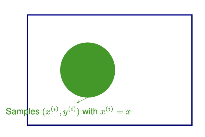
P ^ M L E ( X = x ) = ∑ i = 1 N I ( x ( i ) = x ) N \hat P^{MLE} (X = x) = \frac{\sum^N_{i = 1} \mathbb{I}(x^{(i)} = x)}{N} P ^ M L E ( X = x ) = N ∑ i = 1 N I ( x ( i ) = x )
Given D ∼ P ( Y , X ) \mathcal{D} \sim P(Y, X) D ∼ P ( Y , X ) P ( Y ∣ X ) P(Y | X) P ( Y ∣ X )
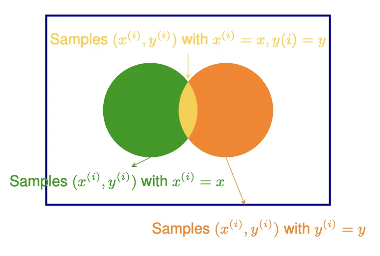
P ^ M L E ( Y = y ∣ X = x ) = P M L E ( Y = y , X = x ) P M L E ( X = x ) = ∑ i = 1 N I ( x ( i ) = x , y ( i ) = y ) ∑ i = 1 N I ( x ( i ) = x ) \begin{align*}
&\hat P^{MLE}(Y = y | X = x) \\
&= \frac{P^{MLE}(Y = y, X = x)}{P^{MLE}(X = x)} \\
&= \frac{\sum^N_{i = 1} \mathbb{I}(x^{(i)} = x, y^{(i)} = y)}{\sum^N_{i = 1} \mathbb{I}(x^{(i)} = x)} \\
\end{align*} P ^ M L E ( Y = y ∣ X = x ) = P M L E ( X = x ) P M L E ( Y = y , X = x ) = ∑ i = 1 N I ( x ( i ) = x ) ∑ i = 1 N I ( x ( i ) = x , y ( i ) = y )
D-dimensional Space
∑ i = 1 N I ( x 1 ( i ) = x 1 , x 2 ( i ) = x 2 , … , x d ( i ) = x d y ( i ) = y ) ∑ i = 1 N I ( x 1 ( i ) = x 1 , x 2 ( i ) = x 2 , … , x d ( i ) = x d ) \frac{\sum^N_{i = 1} \mathbb{I}(x^{(i)}_1 = x_1, x^{(i)}_2 = x_2, \dots, x^{(i)}_d = x_d y^{(i)} = y)}{\sum^N_{i = 1} \mathbb{I}(x^{(i)}_1 = x_1, x^{(i)}_2 = x_2, \dots, x^{(i)}_d = x_d)} \\ ∑ i = 1 N I ( x 1 ( i ) = x 1 , x 2 ( i ) = x 2 , … , x d ( i ) = x d ) ∑ i = 1 N I ( x 1 ( i ) = x 1 , x 2 ( i ) = x 2 , … , x d ( i ) = x d y ( i ) = y )
It is only good if there are many training examples with the same identical features as x for high dimensional space
Suppose X 1 , … , X d X_1, \dots, X_d X 1 , … , X d Y Y Y A n s : 2 d Ans: 2^d A n s : 2 d
Bayes Rule
( ∀ k , j ) P ( Y = y k ∣ X = x j ) = P ( X = x j ∣ Y = y k ) P ( Y = y k ) P ( X = x j ) = P ( Y = y k ∣ X = x j ) P ( X = x j ) P ( X = x j ) \begin{align*}
&(\forall k, j)\quad \\
&P(Y = y_k | X = x_j)\\
&= \frac{P(X = x_j | Y = y_k) P(Y = y_k)}{P(X = x_j)} \\
&= \frac{P(Y = y_k | X = x_j) P(X = x_j)}{P(X = x_j)}
\end{align*} ( ∀ k , j ) P ( Y = y k ∣ X = x j ) = P ( X = x j ) P ( X = x j ∣ Y = y k ) P ( Y = y k ) = P ( X = x j ) P ( Y = y k ∣ X = x j ) P ( X = x j ) Unfortunately Bayes’ Rule Alone Does not Reduce the Parameters Needed
∙ \bullet ∙ P ( Y ∣ X 1 , … , X d ) P(Y \mid X_1, \dots, X_d) P ( Y ∣ X 1 , … , X d ) P ( Y ∣ X 1 , … , X d ) = P ( X 1 , … , X d ∣ Y ) P ( Y ) P ( X 1 , … , X d ) \begin{align*}
P(Y \mid X_1, \dots, X_d) = \frac{P(X_1, \dots, X_d \mid Y)P(Y)}{P(X_1, \dots, X_d)}
\end{align*} P ( Y ∣ X 1 , … , X d ) = P ( X 1 , … , X d ) P ( X 1 , … , X d ∣ Y ) P ( Y ) ∙ \bullet ∙
P ( X 1 , … , X d ∣ Y = 1 ) : 2 d − 1 P(X_1, \dots, X_d \mid Y = 1): 2^d - 1 P ( X 1 , … , X d ∣ Y = 1 ) : 2 d − 1 P ( X 1 , … , X d ∣ Y = 0 ) : 2 d − 1 P(X_1, \dots, X_d \mid Y = 0): 2^d - 1 P ( X 1 , … , X d ∣ Y = 0 ) : 2 d − 1 P ( Y ) : 1 P(Y): 1 P ( Y ) : 1
Therefore, the total of the parameters needed for P ( X ∣ Y ) P(X\mid Y) P ( X ∣ Y ) 2 ( 2 d − 1 ) + 1 2(2^d - 1) + 1 2 ( 2 d − 1 ) + 1 2 d 2^d 2 d
Naive Bayes
Assumption
P ( X 1 , … , X d ∣ Y ) = ∏ j = 1 d P ( X j ∣ Y ) P(X_1, \dots, X_d \mid Y) = \prod^d_{j = 1} P(X_j \mid Y) P ( X 1 , … , X d ∣ Y ) = j = 1 ∏ d P ( X j ∣ Y ) where
X 1 , … , X d X_1, \dots, X_d X 1 , … , X d conditionally independent given Y Y Y
What Is Conditional Independence?
∀ ( j , k , t ) , P ( X = x j ∣ Y = Y k , Z = Z t ) = P ( X = x j ∣ Z = Z t ) \forall (j, k, t), P(X = x_j \mid Y = Y_k, Z = Z_t) = P(X = x_j \mid Z = Z_t) ∀ ( j , k , t ) , P ( X = x j ∣ Y = Y k , Z = Z t ) = P ( X = x j ∣ Z = Z t )
X X X Y Y Y conditionally independent given Z Z Z
Naive Bayes Successfully Reduces the Number of Parameters Needed
∙ \bullet ∙ P ( Y ∣ X 1 , … , X d ) P(Y \mid X_1, \dots, X_d) P ( Y ∣ X 1 , … , X d ) P ( Y ∣ X 1 , … , X d ) = ∏ j = 1 d P ( X j ∣ Y ) P ( Y ) P ( X 1 , … , X d ) P(Y \mid X_1, \dots, X_d) = \frac{\prod^{d}_{j = 1} P(X_j \mid Y)P(Y)}{P(X_1, \dots, X_d)} P ( Y ∣ X 1 , … , X d ) = P ( X 1 , … , X d ) ∏ j = 1 d P ( X j ∣ Y ) P ( Y ) ∙ \bullet ∙
∏ j = 1 d P ( X j ∣ Y = 1 ) : d \prod^d_{j = 1} P(X_j \mid Y = 1): d ∏ j = 1 d P ( X j ∣ Y = 1 ) : d ∏ j = 1 d P ( X j ∣ Y = 0 ) : d \prod^d_{j = 1} P(X_j \mid Y = 0): d ∏ j = 1 d P ( X j ∣ Y = 0 ) : d P ( Y ) = 1 P(Y) = 1 P ( Y ) = 1
The total number of parameters is brought down to 2 d + 1 2d + 1 2 d + 1
For Optimization
P ( Y = y k ∣ X 1 , … , X d ) = ∏ j = 1 d P ( X j ∣ Y = y k ) P ( Y = y k ) P ( X 1 , … , X d ) ∝ P ( Y ) ∏ j = 1 d P ( X j ∣ Y = y k ) ⇒ Y n e w ← arg max y k ( Y = y k ) ∏ j = 1 d P ( X j n e w ∣ Y = y k ) (Given a new instance) \begin{align*}
&P(Y = y_k \mid X_1, \dots, X_d) \\
&= \frac{\prod^d_{j = 1} P(X_j \mid Y = y_k)P(Y = y_k)}{P(X_1, \dots, X_d)} \\
&\propto P(Y) \prod^d_{j = 1} P(X_j \mid Y = y_k) \\
&\Rightarrow Y_{new} \leftarrow \argmax_{y_k} (Y = y_k) \prod^d_{j = 1} P(X^{new}_j \mid Y = y_k) \quad \text{(Given a new instance)}
\end{align*} P ( Y = y k ∣ X 1 , … , X d ) = P ( X 1 , … , X d ) ∏ j = 1 d P ( X j ∣ Y = y k ) P ( Y = y k ) ∝ P ( Y ) j = 1 ∏ d P ( X j ∣ Y = y k ) ⇒ Y n e w ← y k arg max ( Y = y k ) j = 1 ∏ d P ( X j n e w ∣ Y = y k ) (Given a new instance) Naive Bayes - Discrete Features
X j ∈ { 1 , 2 , … , K j } , ∀ j ∈ { 1 , 2 , … , d } Y ∈ { 1 , 2 , … , C } P ( X j = k ∣ Y = c ) = θ j k c \begin{align*}
X_j &\in \{1, 2, \dots, K_j\}, \forall j \in \{1, 2, \dots, d\} \\
Y &\in \{1, 2, \dots, C\} \\
P(X_j = k \mid Y = c) &= \theta_{jkc}
\end{align*} X j Y P ( X j = k ∣ Y = c ) ∈ { 1 , 2 , … , K j } , ∀ j ∈ { 1 , 2 , … , d } ∈ { 1 , 2 , … , C } = θ jk c where
∑ k = 1 K j θ j k c = 1 \sum^{K_j}_{k = 1} \theta_{jkc} = 1 ∑ k = 1 K j θ jk c = 1
The sum of the probability of feature j equal to k given the label c is 1 \text{The sum of the probability of feature j equal to k given the label c is 1} The sum of the probability of feature j equal to k given the label c is 1 Maximum Likelihood Estimates (MLE)
Prior
π ^ c M L E = P ^ M L E ( Y = c ) = # of samples in class c # of samples = ∑ i = 1 N I { y ( i ) = c } N \begin{align*}
\hat{\pi}^{MLE}_c &= \hat{P}^{MLE} (Y = c) \\
&= \frac{\# \text{ of samples in class c}}{\# \text{ of samples}} \\
&= \frac{\sum^{N}_{i = 1} \mathbb{I}\{y^{(i)} = c\}}{N}
\end{align*} π ^ c M L E = P ^ M L E ( Y = c ) = # of samples # of samples in class c = N ∑ i = 1 N I { y ( i ) = c } hallucinated Prior
π ^ c M L E = ∑ i = 1 N I { y ( i ) = c } + l N + l c \hat{\pi}^{MLE}_c = \frac{\sum^{N}_{i = 1} \mathbb{I}\{y^{(i)} = c\} + l}{N + lc} π ^ c M L E = N + l c ∑ i = 1 N I { y ( i ) = c } + l Likelihood
θ ^ j k c M L E = P ^ M L E ( X j = k ∣ Y = c ) = # of samples with the label c and have feature X j = k # of samples with the label c = ∑ i = 1 N I { y ( i ) = c ∩ x j ( i ) = k } ∑ i = 1 N I { y ( i ) = c } \begin{align*}
\hat{\theta}^{MLE}_{jkc} &= \hat{P}^{MLE}(X_j = k \mid Y = c) \\
&= \frac{\# \text{ of samples with the label c and have feature }X_j = k}{\# \text{ of samples with the label c}} \\
&= \frac{\sum^{N}_{i = 1} \mathbb{I}\{y^{(i)} = c \cap x^{(i)}_j = k\}}{\sum^{N}_{i = 1} \mathbb{I}\{y^{(i)} = c\}}
\end{align*} θ ^ jk c M L E = P ^ M L E ( X j = k ∣ Y = c ) = # of samples with the label c # of samples with the label c and have feature X j = k = ∑ i = 1 N I { y ( i ) = c } ∑ i = 1 N I { y ( i ) = c ∩ x j ( i ) = k } Hallucinated Likelihood
θ ^ j k c M L E = ∑ i = 1 N I { y ( i ) = c ∩ x j ( i ) = k } + l ∑ i = 1 N I { y ( i ) = c } + l K j \hat{\theta}^{MLE}_{jkc} = \frac{\sum^{N}_{i = 1} \mathbb{I}\{y^{(i)} = c \cap x^{(i)}_j = k\} + l}{\sum^{N}_{i = 1} \mathbb{I}\{y^{(i)} = c\} + lK_j} θ ^ jk c M L E = ∑ i = 1 N I { y ( i ) = c } + l K j ∑ i = 1 N I { y ( i ) = c ∩ x j ( i ) = k } + l Learning to Classify Documents: P ( Y ∣ X ) P(Y \mid X) P ( Y ∣ X )
Question
Given a document of length M M M
Y Y Y X = < X 1 , … , X d > X = <X_1, \dots, X_d> X =< X 1 , … , X d > ∀ j ∈ { 1 , 2 , … , d } \forall j \in \{1, 2, \dots, d\} ∀ j ∈ { 1 , 2 , … , d } X j X_j X j
I am pleased to announce that Bob Frederking of the Language
Technologies Institute is our new Associate Dean for Graduate
Programs. In this role, he oversees the many issues that arise
with our multiple masters and PhD programs. Bob brings to this
positions considerable expereince with the masters and PhD
programs in the LTI.

I would like to thank Frank Pfenning, who has served ably in this
role for the past two years.
Answer
d : d: d : X j : X_j: X j : j j j M = ∑ j = 1 d X j M = \sum^d_{j = 1} X_j M = ∑ j = 1 d X j
∙ \bullet ∙ P ( X ∣ M , Y = c ) = M ! X 1 ! X 2 ! ⋯ X d ! ∏ j = 1 d ( θ j c ) X j P(X \mid M, Y = c) = \frac{M!}{X_1!X_2! \cdots X_d!} \prod_{j = 1}^{d} (\theta_{jc})^{X_j} P ( X ∣ M , Y = c ) = X 1 ! X 2 ! ⋯ X d ! M ! j = 1 ∏ d ( θ j c ) X j where
θ j c \theta_{jc} θ j c j j j ∑ j = 1 d θ j c = 1 \sum^d_{j = 1} \theta_{jc} = 1 ∑ j = 1 d θ j c = 1 ∏ j = 1 d ( θ j c ) X j \prod_{j = 1}^{d} (\theta_{jc})^{X_j} ∏ j = 1 d ( θ j c ) X j The product of the probabilities ( θ j c ) (\theta_{jc}) ( θ j c ) ( X j ) (X_j) ( X j )
The probability of a pattern occurs under label Y = c Y = c Y = c
M ! X 1 ! X 2 ! ⋯ X d ! \frac{M!}{X_1!X_2! \cdots X_d!} X 1 ! X 2 ! ⋯ X d ! M ! 1 X 1 ! X 2 ! ⋯ X d ! \frac{1}{X_1!X_2!\cdots X_d!} X 1 ! X 2 ! ⋯ X d ! 1 the permutation of the pattern
∙ \bullet ∙ θ ^ j c M L E = # of times word j appears in emails with label c # of words in all emails with lable c = ∑ i = 1 N I { y ( i ) = c } x j ( i ) ∑ i = 1 N I { y ( i ) = c } ∑ v = 1 d x v ( i ) \begin{align*}
\hat{\theta}_{jc}^{MLE} &= \frac{\# \text{of times word j appears in emails with label c}}{\# \text{of words in all emails with lable c}} \\
&= \frac{\sum^N_{i = 1}\mathbb{I}\{y^{(i) } = c\}x_j^{(i)}}{\sum^{N}_{i = 1} \mathbb{I}\{y^{(i)} = c\}\sum^d_{v = 1} x_v^{(i)}} \\
\end{align*} θ ^ j c M L E = # of words in all emails with lable c # of times word j appears in emails with label c = ∑ i = 1 N I { y ( i ) = c } ∑ v = 1 d x v ( i ) ∑ i = 1 N I { y ( i ) = c } x j ( i ) ∙ \bullet ∙ θ ^ j c M A P = ∑ i = 1 N I { y ( i ) = c } x j ( i ) + β j c ∑ i = 1 N I { y ( i ) = c } ∑ v = 1 N x v ( i ) + ∑ v = 1 d β v c \hat{\theta}^{MAP}_{jc} = \frac{\sum^N_{i = 1}\mathbb{I}\{y^{(i) } = c\}x_j^{(i)} + \beta_{jc}}{\sum^{N}_{i = 1} \mathbb{I}\{y^{(i)} = c\}\sum^N_{v = 1}x^{(i)}_v + \sum^d_{v = 1}\beta_{vc}} θ ^ j c M A P = ∑ i = 1 N I { y ( i ) = c } ∑ v = 1 N x v ( i ) + ∑ v = 1 d β v c ∑ i = 1 N I { y ( i ) = c } x j ( i ) + β j c
Here β \beta β
β = 1 \beta = 1 β = 1
Continuous Data
For continuous data, we assume that the Likelihood follows the Gaussian Distribution
P ( Y = c ∣ X 1 , … , X d ) = P ( Y = c ) ∏ j = 1 d P ( X j ∣ Y = c ) ∑ k = 1 C P ( Y = k ) ∑ j = 1 d P ( X j ∣ Y = k ) P(Y = c \mid X_1, \dots, X_d) = \frac{P(Y = c)\prod^d_{j = 1} P(X_j\mid Y = c)}{\sum^C_{k = 1} P(Y = k)\sum^d_{j = 1} P(X_j \mid Y = k)} P ( Y = c ∣ X 1 , … , X d ) = ∑ k = 1 C P ( Y = k ) ∑ j = 1 d P ( X j ∣ Y = k ) P ( Y = c ) ∏ j = 1 d P ( X j ∣ Y = c ) where
P ( X j ∣ Y = c ) ∼ N ( μ , σ 2 ) P(X_j \mid Y = c) \sim N(\mu, \sigma^2) P ( X j ∣ Y = c ) ∼ N ( μ , σ 2 )
Normal Distribution
p ( x ) ∼ N ( μ , σ 2 ) = 1 2 π σ 2 e − 1 2 ( x − μ σ ) 2 p(x) \sim N(\mu, \sigma^2) = \frac{1}{\sqrt{2\pi\sigma^2}} e^{-\frac{1}{2}(\frac{x - \mu}{\sigma})^2} p ( x ) ∼ N ( μ , σ 2 ) = 2 π σ 2 1 e − 2 1 ( σ x − μ ) 2 where
∫ a b p ( x ) d x = 1 \int^b_a p(x) dx = 1 ∫ a b p ( x ) d x = 1
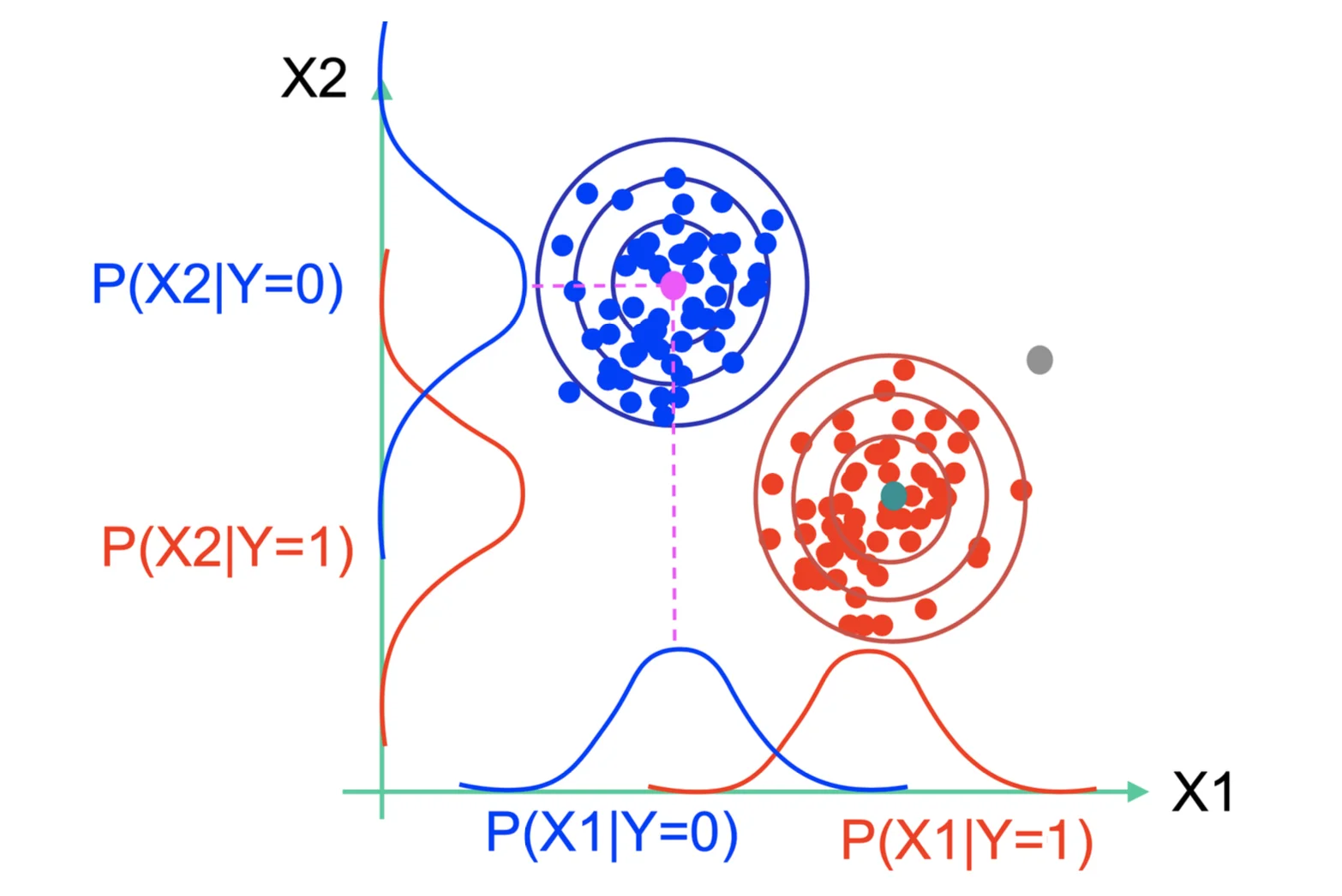
Gaussian Naive Bayes (GNB)
P ( X j = x ∣ Y = c ) = 1 2 π σ j c 2 e − 1 2 ( x − μ j c σ j c ) 2 P(X_j = x\mid Y = c) = \frac{1}{\sqrt{2\pi\sigma^2_{jc}}} e^{-\frac{1}{2}(\frac{x - \mu_{jc}}{\sigma_{jc}})^2} P ( X j = x ∣ Y = c ) = 2 π σ j c 2 1 e − 2 1 ( σ j c x − μ j c ) 2
Sometimes, we assume X j X_j X j Y Y Y σ j c 2 \sigma^2_{jc} σ j c 2
Estimating Parameters: Discrete Y, Continuous X
Given dataset: { x ( i ) , y ( i ) } i = 1 N \{x^{(i)}, y^{(i)}\}_{i =1}^N { x ( i ) , y ( i ) } i = 1 N
x ( i ) ∈ R d x^{(i)} \in \R^d x ( i ) ∈ R d y ( i ) ∈ R y^{(i)} \in \R y ( i ) ∈ R j j j i i i c c c
∙ \bullet ∙ μ ^ j c \hat{\mu}_{jc} μ ^ j c μ ^ j c = 1 ∑ i = 1 N I { y ( i ) = c } ∑ i = 1 N x j ( i ) I { y ( i ) = c } \hat{\mu}_{jc} = \frac{1}{\sum^N_{i = 1} \mathbb{I}\{y^{(i)} = c\}} \sum^{N}_{i = 1} x_j^{(i)} \mathbb{I}\{y^{(i)} = c\} μ ^ j c = ∑ i = 1 N I { y ( i ) = c } 1 i = 1 ∑ N x j ( i ) I { y ( i ) = c } ∙ \bullet ∙ σ ^ j c 2 \hat{\sigma}_{jc}^2 σ ^ j c 2 σ ^ j c 2 = 1 ∑ i = 1 N I { y ( i ) = c } ∑ i = 1 N ( x j ( i ) − μ ^ j c ) 2 I { y ( i ) = c } \hat{\sigma}_{jc}^2 = \frac{1}{\sum^N_{i = 1} \mathbb{I}\{y^{(i)} = c\}} \sum^N_{i =1} (x_j^{(i)} - \hat{\mu}_{jc})^2 \mathbb{I}\{y^{(i)} = c\} σ ^ j c 2 = ∑ i = 1 N I { y ( i ) = c } 1 i = 1 ∑ N ( x j ( i ) − μ ^ j c ) 2 I { y ( i ) = c } If variance of each feature is independent of classes
Y n e w ← arg max y ∈ { 0 , 1 } P ( Y = y ) ∏ j = 1 d P ( X j n e w ∣ Y = y ) Y_{new} \leftarrow \argmax_{y \in \{0, 1\}} P(Y =y)\prod^d_{j = 1} P(X^{new}_j\mid Y = y) Y n e w ← y ∈ { 0 , 1 } arg max P ( Y = y ) j = 1 ∏ d P ( X j n e w ∣ Y = y )
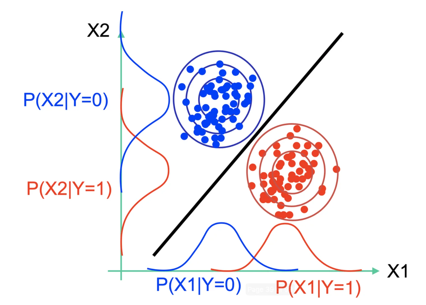
Decision Boundary
The decision boundary occurs where P ( Y = 0 ) ∏ j = 1 d P ( X j ∣ Y = 0 ) = P ( Y = 1 ) ∏ j = 1 d P ( X j ∣ Y = 1 ) P(Y = 0) \prod^d_{j = 1}P(X_j \mid Y = 0) = P(Y =1) \prod^d_{j =1} P(X_j \mid Y= 1) P ( Y = 0 ) ∏ j = 1 d P ( X j ∣ Y = 0 ) = P ( Y = 1 ) ∏ j = 1 d P ( X j ∣ Y = 1 )
Multinomial Naive Bayes
When is an input data classified with label 1?
P ( Y = 1 ∣ X ) > P ( Y = 0 ∣ X ) ⟺ P ( Y = 1 ∣ X ) > P ( Y = 0 ∣ X ) ⟺ P ( X ∣ Y = 1 ) P ( Y = 1 ) > P ( X ∣ Y = 0 ) P ( Y = 0 ) ⟺ M ! X 1 ! X 2 ! ⋯ X d ! ∏ j = 1 d ( θ j 1 ) X j P ( Y = 1 ) > M ! X 1 ! X 2 ! ⋯ X d ! ∏ j = 1 d ( θ j 0 ) X j P ( Y = 0 ) ⟺ ∏ j = 1 d ( θ j 1 ) X j P ( Y = 1 ) > ∏ j = 1 d ( θ j 0 ) X j P ( Y = 0 ) ⟺ ∑ j = 1 d X j ln ( θ j 1 ) + ln P ( Y = 1 ) > ∑ j = 1 d X j ln ( θ j 0 ) + ln P ( Y = 0 ) ⟺ ∑ j = 1 d X j ( ln ( θ j 1 ) − ln ( θ j 0 ) ) + ln P ( Y = 1 ) − ln P ( Y = 0 ) > 0 l e t w 0 = ln P ( Y = 1 ) − ln P ( Y = 0 ) , w j = ( ln ( θ j 1 ) − ln ( θ j 0 ) ) ⟺ w 0 + ∑ j = 1 d X j w j > 0 ( A linear classifier ) \begin{align*}
&P(Y = 1 \mid X) > P(Y = 0 \mid X) \\
&\iff P(Y = 1 \mid X) > P(Y = 0 \mid X) \\
&\iff P(X\mid Y = 1) P(Y = 1) > P(X \mid Y = 0 ) P(Y = 0) \\
&\iff \frac{M!}{X_1!X_2!\cdots X_d!} \prod^d_{j = 1} (\theta_{j1})^{X_j} P(Y = 1) > \frac{M!}{X_1!X_2!\cdots X_d!} \prod^d_{j = 1} (\theta_{j0})^{X_j} P(Y = 0) \\
&\iff \prod^d_{j = 1} (\theta_{j1})^{X_j} P(Y = 1) > \prod^d_{j = 1} (\theta_{j0})^{X_j} P(Y = 0) \\
&\iff \sum^d_{j = 1} {X_j}\ln(\theta_{j1}) + \ln P(Y = 1) > \sum^d_{j = 1} {X_j}\ln(\theta_{j0}) + \ln P(Y = 0) \\
&\iff \sum^d_{j = 1} {X_j}(\ln(\theta_{j1}) - \ln(\theta_{j0})) + \ln P(Y = 1) - \ln P(Y = 0) > 0 \\
&let\ w_0 = \ln P(Y = 1) - \ln P(Y = 0),\ w_j = (\ln(\theta_{j1}) - \ln(\theta_{j0})) \\
&\iff w_0 + \sum^d_{j = 1} X_jw_j > 0 \quad (\text{A linear classifier})
\end{align*} P ( Y = 1 ∣ X ) > P ( Y = 0 ∣ X ) ⟺ P ( Y = 1 ∣ X ) > P ( Y = 0 ∣ X ) ⟺ P ( X ∣ Y = 1 ) P ( Y = 1 ) > P ( X ∣ Y = 0 ) P ( Y = 0 ) ⟺ X 1 ! X 2 ! ⋯ X d ! M ! j = 1 ∏ d ( θ j 1 ) X j P ( Y = 1 ) > X 1 ! X 2 ! ⋯ X d ! M ! j = 1 ∏ d ( θ j 0 ) X j P ( Y = 0 ) ⟺ j = 1 ∏ d ( θ j 1 ) X j P ( Y = 1 ) > j = 1 ∏ d ( θ j 0 ) X j P ( Y = 0 ) ⟺ j = 1 ∑ d X j ln ( θ j 1 ) + ln P ( Y = 1 ) > j = 1 ∑ d X j ln ( θ j 0 ) + ln P ( Y = 0 ) ⟺ j = 1 ∑ d X j ( ln ( θ j 1 ) − ln ( θ j 0 )) + ln P ( Y = 1 ) − ln P ( Y = 0 ) > 0 l e t w 0 = ln P ( Y = 1 ) − ln P ( Y = 0 ) , w j = ( ln ( θ j 1 ) − ln ( θ j 0 )) ⟺ w 0 + j = 1 ∑ d X j w j > 0 ( A linear classifier ) Multinomial Gaussian Bayes
Consider f : X → Y f: X \rightarrow Y f : X → Y
X X X < X 1 , … , X d > <X_1, \dots, X_d> < X 1 , … , X d > Y Y Y Assume all X j X_j X j Y Y Y
Model P ( X j ∣ Y = c ) ∼ N ( μ j c , σ j 2 ) P(X_j \mid Y = c) \sim \mathcal{N}(\mu_{jc}, \sigma^2_{j}) P ( X j ∣ Y = c ) ∼ N ( μ j c , σ j 2 )
Model P ( Y ) ∼ B e r n o u l l i ( π ) P(Y) \sim Bernoulli(\pi) P ( Y ) ∼ B er n o u ll i ( π )
P ( Y = 0 ∣ X ) = P ( Y = 0 ) P ( X ∣ Y = 0 ) P ( Y = 0 ) P ( X ∣ Y = 0 ) + P ( Y = 1 ) P ( X ∣ Y = 1 ) = 1 1 + P ( Y = 1 ) P ( X ∣ Y = 1 ) P ( Y = 0 ) P ( X ∣ Y = 0 ) = 1 1 + π P ( X ∣ Y = 1 ) ( 1 − π ) P ( X ∣ Y = 0 ) = 1 1 + exp ( ln π ( 1 − π ) + ln P ( X ∣ Y = 1 ) P ( X ∣ Y = 0 ) ) = 1 1 + exp ( ln π ( 1 − π ) + ∑ j = 1 d ( ln exp ( − ( X j − μ j 1 ) 2 2 σ j 2 ) exp ( − ( X j − μ j 0 ) 2 2 σ j 2 ) ) ) ( 1 2 π σ j 2 exp ( − ( X j − μ j c 2 σ j ) 2 ) = 1 1 + exp ( ln π ( 1 − π ) + ∑ j = 1 d ( − X j 2 + 2 X j μ j 1 − μ j 1 2 σ j 2 ) + ( X j 2 − 2 X j μ j 1 μ j 1 2 σ j 2 ) ) = 1 1 + exp ( ln π ( 1 − π ) + ∑ j = 1 d ( − X j 2 + 2 X j μ j 1 − μ j 1 2 σ j 2 ) + ( X j 2 − 2 X j μ j 1 μ j 1 2 σ j 2 ) ) = 1 1 + exp ( ln π ( 1 − π ) + ∑ j = 1 d ( X j ( μ j 1 − μ j 0 ) σ j 2 ) + ( μ j 0 2 − μ j 1 2 σ j 2 ) ) = 1 1 + exp ( ln π ( 1 − π ) + ∑ j = 1 d μ j 0 2 − μ j 1 2 σ j 2 + ∑ j = 1 d X j ( μ j 1 − μ j 0 ) σ j 2 ) let w 0 = ln π ( 1 − π ) + ∑ j = 1 d μ j 0 2 − μ j 1 2 σ j 2 w j = ∑ j = 1 d X j ( μ j 1 − μ j 0 ) σ j 2 = 1 1 + e w 0 + ∑ j = 1 d w j X j P ( Y = 1 ∣ X ) = 1 − 1 1 + e w 0 + ∑ j = 1 d w j X j = e w 0 + ∑ j = 1 d w j X j 1 + e w 0 + ∑ j = 1 d w j X j ⇒ P ( Y = 1 ∣ X ) P ( Y = 0 ∣ X ) = e w 0 + ∑ j = 1 d w j X j ≷ 1 ⇒ ln P ( Y = 1 ∣ X ) P ( Y = 0 ∣ X ) = w 0 + ∑ j = 1 d w j X j ≷ 0 (Linear Classification Rule) \begin{align*}
&\begin{align*}
P(Y = 0 \mid X) &= \frac{P(Y = 0)P(X \mid Y = 0)}{P(Y = 0)P(X \mid Y = 0) + P(Y = 1) P(X \mid Y = 1)} \\
&= \frac{1}{1 + \frac{P(Y = 1) P(X \mid Y = 1)}{P(Y = 0)P(X \mid Y = 0)}} \\
&= \frac{1}{1 + \frac{\pi P(X \mid Y = 1)}{(1 - \pi)P(X \mid Y = 0)}} \\
&= \frac{1}{1 + \exp (\ln \frac{\pi}{(1 - \pi)} + \ln\frac{P(X \mid Y = 1)}{P(X \mid Y = 0)})} \\
&= \frac{1}{1 + \exp (\ln \frac{\pi}{(1 - \pi)} + \sum^{d}_{j = 1} (\ln \frac{\exp(\frac{- (X_j - \mu_{j1})^2}{2\sigma^2_j})}{\exp(\frac{- (X_j - \mu_{j0})^2}{2\sigma^2_j})}))} \quad\quad (\frac{1}{\sqrt{2\pi\sigma_j^2}} \exp(- (\frac{X_j - \mu_{jc}}{\sqrt{2}\sigma_{j}})^2) \\
&= \frac{1}{1 + \exp (\ln \frac{\pi}{(1 - \pi)} + \sum^{d}_{j = 1} (\frac{-X_j^2 + 2X_j\mu_{j1} - \mu^2_{j1}}{\sigma^2_j})+ (\frac{X_j^2 - 2X_j\mu_{j1} \mu^2_{j1}}{\sigma^2_j}))} \\
&= \frac{1}{1 + \exp (\ln \frac{\pi}{(1 - \pi)} + \sum^{d}_{j = 1} (\frac{\cancel{-X_j^2} + 2X_j\mu_{j1} - \mu^2_{j1}}{\sigma^2_j})+ (\frac{\cancel{X_j^2} - 2X_j\mu_{j1} \mu^2_{j1}}{\sigma^2_j}))} \\
&= \frac{1}{1 + \exp (\ln \frac{\pi}{(1 - \pi)} + \sum^{d}_{j = 1} (X_j\frac{(\mu_{j1} - \mu_{j0})}{\sigma^2_j})+ (\frac{\mu_{j0}^2 - \mu_{j1}^2}{\sigma^2_j}))} \\
&= \frac{1}{1 + \exp (\ln \frac{\pi}{(1 - \pi)} + \sum^{d}_{j = 1} \frac{\mu_{j0}^2 - \mu_{j1}^2}{\sigma^2_j}+ \sum^{d}_{j = 1} X_j\frac{(\mu_{j1} - \mu_{j0})}{\sigma^2_j})} \\
\text{let } &w_0 = \ln \frac{\pi}{(1 - \pi)} + \sum^{d}_{j = 1} \frac{\mu_{j0}^2 - \mu_{j1}^2}{\sigma^2_j} \\
&w_j = \sum^{d}_{j = 1} X_j\frac{(\mu_{j1} - \mu_{j0})}{\sigma^2_j} \\
&= \frac{1}{1 + e^{w_0 + \sum^d_{j = 1} w_j X_j}}
\end{align*} \\
&\begin{align*}
P(Y = 1 \mid X) &= 1 - \frac{1}{1 + e^{w_0 + \sum^d_{j = 1} w_j X_j}} \\
&= \frac{e^{w_0 + \sum^d_{j = 1} w_j X_j}}{1 + e^{w_0 + \sum^d_{j = 1} w_j X_j}} \\
\end{align*} \\
&\Rightarrow \frac{P(Y = 1 \mid X)}{P(Y = 0 \mid X)} = e^{w_0 + \sum^d_{j = 1} w_j X_j} \gtrless 1 \\
&\Rightarrow \ln \frac{P(Y = 1 \mid X)}{P(Y = 0 \mid X)} = w_0 + \sum^d_{j = 1} w_j X_j \gtrless 0 \quad\quad \text{(Linear Classification Rule)}
\end{align*} P ( Y = 0 ∣ X ) let = P ( Y = 0 ) P ( X ∣ Y = 0 ) + P ( Y = 1 ) P ( X ∣ Y = 1 ) P ( Y = 0 ) P ( X ∣ Y = 0 ) = 1 + P ( Y = 0 ) P ( X ∣ Y = 0 ) P ( Y = 1 ) P ( X ∣ Y = 1 ) 1 = 1 + ( 1 − π ) P ( X ∣ Y = 0 ) π P ( X ∣ Y = 1 ) 1 = 1 + exp ( ln ( 1 − π ) π + ln P ( X ∣ Y = 0 ) P ( X ∣ Y = 1 ) ) 1 = 1 + exp ( ln ( 1 − π ) π + ∑ j = 1 d ( ln e x p ( 2 σ j 2 − ( X j − μ j 0 ) 2 ) e x p ( 2 σ j 2 − ( X j − μ j 1 ) 2 ) )) 1 ( 2 π σ j 2 1 exp ( − ( 2 σ j X j − μ j c ) 2 ) = 1 + exp ( ln ( 1 − π ) π + ∑ j = 1 d ( σ j 2 − X j 2 + 2 X j μ j 1 − μ j 1 2 ) + ( σ j 2 X j 2 − 2 X j μ j 1 μ j 1 2 )) 1 = 1 + exp ( ln ( 1 − π ) π + ∑ j = 1 d ( σ j 2 − X j 2 + 2 X j μ j 1 − μ j 1 2 ) + ( σ j 2 X j 2 − 2 X j μ j 1 μ j 1 2 )) 1 = 1 + exp ( ln ( 1 − π ) π + ∑ j = 1 d ( X j σ j 2 ( μ j 1 − μ j 0 ) ) + ( σ j 2 μ j 0 2 − μ j 1 2 )) 1 = 1 + exp ( ln ( 1 − π ) π + ∑ j = 1 d σ j 2 μ j 0 2 − μ j 1 2 + ∑ j = 1 d X j σ j 2 ( μ j 1 − μ j 0 ) ) 1 w 0 = ln ( 1 − π ) π + j = 1 ∑ d σ j 2 μ j 0 2 − μ j 1 2 w j = j = 1 ∑ d X j σ j 2 ( μ j 1 − μ j 0 ) = 1 + e w 0 + ∑ j = 1 d w j X j 1 P ( Y = 1 ∣ X ) = 1 − 1 + e w 0 + ∑ j = 1 d w j X j 1 = 1 + e w 0 + ∑ j = 1 d w j X j e w 0 + ∑ j = 1 d w j X j ⇒ P ( Y = 0 ∣ X ) P ( Y = 1 ∣ X ) = e w 0 + ∑ j = 1 d w j X j ≷ 1 ⇒ ln P ( Y = 0 ∣ X ) P ( Y = 1 ∣ X ) = w 0 + j = 1 ∑ d w j X j ≷ 0 (Linear Classification Rule)
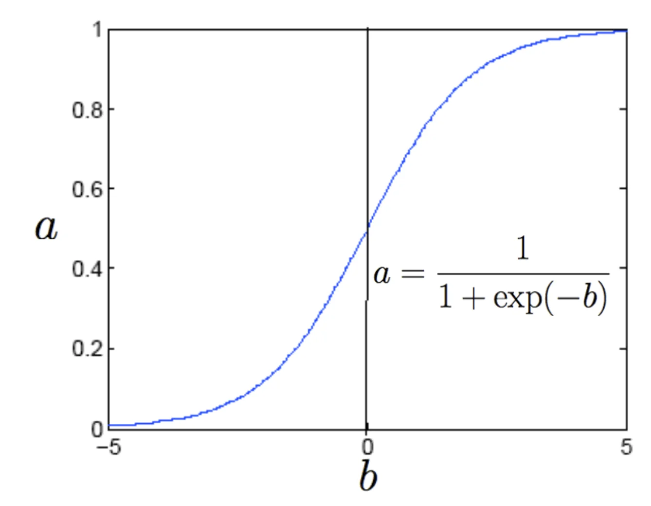
This is the Logistic Function :
1 1 + e w 0 + ∑ j = 1 d w j X j \frac{1}{1 + e^{w_0 + \sum^d_{j = 1} w_jX_j}} 1 + e w 0 + ∑ j = 1 d w j X j 1
Aspect Logistic Regression Naive Bayes Type of model Discriminative — models P ( Y ∣ X ) P(Y \mid X) P ( Y ∣ X ) Generative — models P ( X ∣ Y ) P(X \mid Y) P ( X ∣ Y ) P ( Y ) P(Y) P ( Y ) P ( Y ∣ X ) P(Y \mid X) P ( Y ∣ X ) Key assumption No independence assumption between features Conditional independence of features given the class Decision boundary Linear in feature space (unless nonlinear terms added) Linear if equal variances (e.g., Gaussian NB), otherwise nonlinear Output Direct estimate of P ( Y = 1 ∣ X ) P(Y=1 \mid X) P ( Y = 1 ∣ X ) Computed from P ( X ∣ Y ) P ( Y ) P(X \mid Y) P(Y) P ( X ∣ Y ) P ( Y ) Interpretability Coefficients show log-odds effect of features Parameters correspond to class-conditional feature distributions Data requirement Needs more data for stable estimates Performs well even with small datasets Handling correlated features Can handle correlations and interactions Breaks down if features are correlated Training speed Slower — requires iterative optimization Very fast — closed-form parameter estimation Probability calibration Usually well-calibrated probabilities Often overconfident, may need calibration Regularization Supports L1/L2 regularization Usually no regularization (can add smoothing) Common variants L1/L2 Logistic Regression, Multinomial LR Gaussian NB, Multinomial NB, Bernoulli NB Typical use cases Continuous or mixed data, interpretability needed Text classification, spam detection, sentiment analysis