6. Empirical Risk Minimization (ERM)
Recall: SVM
w,bmin21∣∣w∣∣22+Ci=1∑Nmax(0,1−y(i)(w⊺x(i)+b))
- ∣∣w∣∣22
- regularizer
- ∑i=1Nmax(0,1−y(i)(w⊺x(i)+b))
- loss
Rewrite
wminN1i=1∑NHinge Lossmax(1−y(i)(hw(x(i))w⊺x(i)+b),0)+λL2−Regularizer∣∣w∣∣22
Tip
Check out more on SVM in 5. SVM
Loss Function
wminN1i=1∑Nl(hw(x(i)),y(i))+λr(w)
- The loss function l(hw(x),y) quantifies how badly the estimate hw(x) approximates the real y
- Smaller value → good approximation
Risk
wminN1i=1∑Nl(hw(x(i)),y(i))+λr(w)
- R(h)=EX,Y[l(h(X),Y)]
- Risk of a prediction function h
Warning
How can we minimize the risk without knowing the true distribution.
Empirical Risk Minimization (ERM)
wminempirical riskN1i=1∑Nlossl(hw(x(i)),y(i))
- empirical risk (EM) is the average loss over all the data points
- ERM is a general method to bring down the empirical risk
- Choose w by attempting to match given dataset well, as measured by the loss l
An example of a very poor predictor
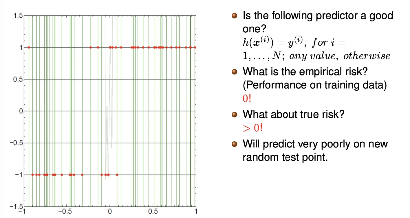
- Does not generalize at all since h(x(i))=y(i)
Regularized Empirical Risk Minimization
wminN1i=1∑Nl(hw(x(i)),y(i))+λr(w)
- When λ=0, RERM becomes ERM
Commonly used Binary Classification Loss Function
y∈{−1,1}
∙ Hinge Loss
max[1−y(i)hw(x(i)),0]p
- p = 1: standard SVM
- p = 2: squared hingeless SVM
∙ Log Loss
log(1+e−y(i)hw(x(i)))
- Logistic regression
- outputs are well-calibrated probabilities
∙ Exponential Loss
e−y(i)hw(x(i))
- AdaBoost
- Mis-prediction can lead to exponential loss
- Nice convergence result but fail to handle noisy data well.
∙ Zero-One Loss
I(hw(x(i))=y(i))I(e){1(e is False)0(e is True)
- Actual classification loss
- Non-continuous and impractical to optimize
Plots
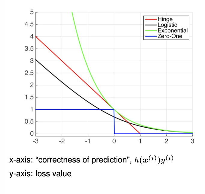
- Hinge Loss and Exponential Loss are the upper bounds of the zero-one loss
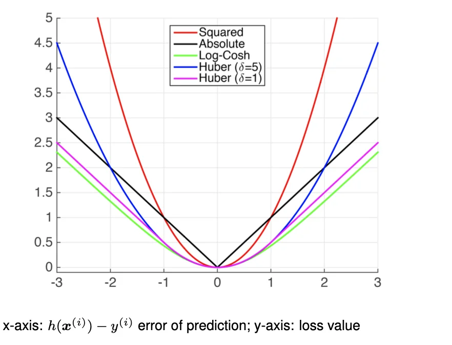
Commonly Used Regression Loss Functions
y∈R1
∙ Squared Loss
(hw(x(i))−y(i))2
- Most popular
- Also known as Ordinary Least Squares (OLS)
- Estimates mean label
- Pros:
- differentiable everywhere
- Cons:
- sensitive to outliers/noise
∙ Absolute Loss
∣hw(x(i))−y(i)∣
- Estimates median label
- Pros:
- Less sensitive to noises
- Cons:
- Not differentiable at 0
∙ Huber Loss
{21(hw(x(i))−y(i))2(∣hw(x(i))−y(i)>δ∣)δ(∣hw(x(i)−y(i))∣−2δ)(otherwise)
- Also known as Smooth Absolute Loss
- Set a threshold δ
- loss>δ: Large error, absolute loss
- loss<δ: Small error, squared loss
∙ Log-cosh loss
log(cosh(hw(x(i))−y(i)))
where
cosh(x)=2ex+e−x
Plots
Regularizers
wminN1i=1∑Nl(hw(x(i)),y(i))−λr(w)⟺wminN1i=1∑Nl(hw(x(i)),y(i))s.t.r(w)≤B
- ∀λ,λ≥0⟹∃B≥0 s.t. the above formulations hold
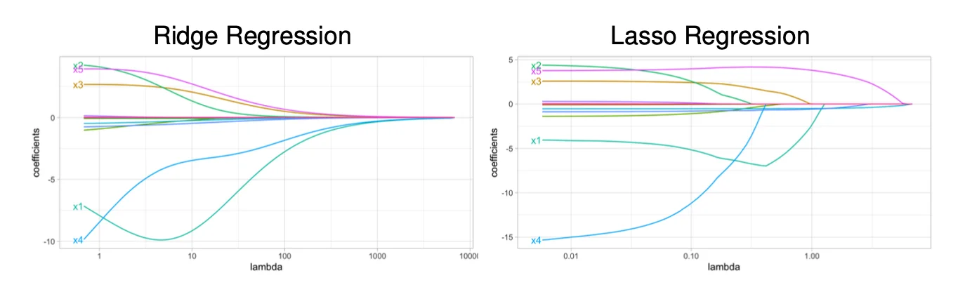
Types of Regularizers
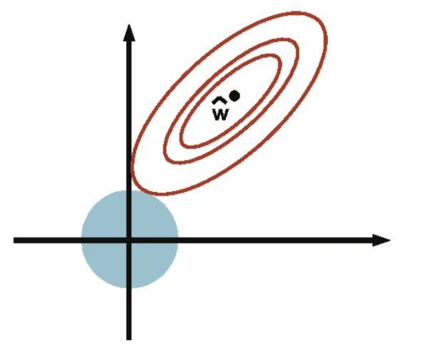
l2−regularization

r(w)=w⊺w=∣∣w∣∣22
- strictly convex (+)
- differentiable (+)
- uses weights on all features (-)
l1−regularization
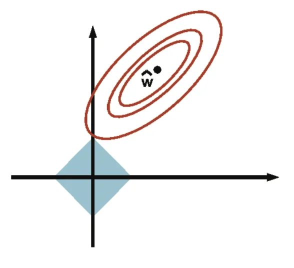
r(w)=∣∣w∣∣1
- convex (but not strictly)
- not differentiable at 0 (minimization intends to bring us to)
- sparse (most of its elements are zeros)
lp−regularization
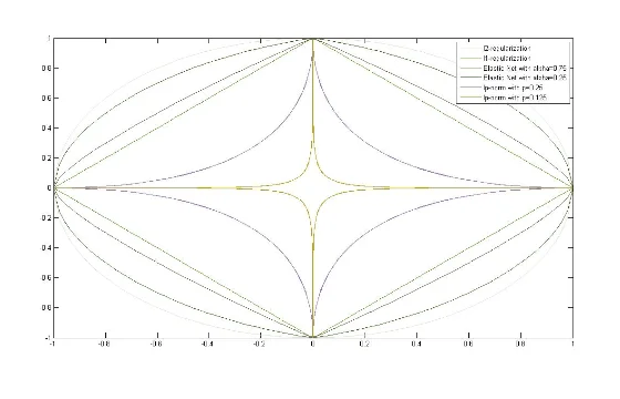
r(w)=∣∣w∣∣p=(i=1∑Nwip)p1
- non-convex (-)
- very-sparse solutions (+)
- initialization-dependent
- not differentiable (-)
Elastic Net
- The combination of Lasso (L1) and Ridge (L2) regressions
wminN1i=1∑N(w⊺x(i)−y(i))2+α∣∣w∣∣1+(1−α)∣∣w∣∣22
- strictly convex
- sparsity inducing
- non-differentiable